PFS Go/Nogo design
PFS_Gonogo.RmdNote: This vignette, including functions for TTE Go/Nogo design, are still under development. Hence they are subject to possible change in the future.
library(gonogo)
library(dplyr)
#>
#> Attaching package: 'dplyr'
#> The following objects are masked from 'package:stats':
#>
#>     filter, lag
#> The following objects are masked from 'package:base':
#>
#>     intersect, setdiff, setequal, union
library(tidyr)
library(ggplot2)
library(ggrepel)
# require(cowplot)
# require(survival)
library(future.apply)
#> Loading required package: future
library(progressr)

# number of parallel cores,
# please adjust according to your machine's capability
# current setting is to leave (at most) 2 cores not used, since the function
#   is guaranteed to return at least 1 core for later parallel computation.
worker_num <- parallelly::availableCores(omit = 2)
plan(cluster, workers = worker_num)

# progress info report settings
handlers("cli")
progress_interval <- 50

# fix the seed for random number generation
# Note that later the RNG kind will be set to a parallel safe one
random_seed <- 1024
Basic Settings
In this article, an example of Go/Nogo design based on PFS is demonstrated. First we need some settings about this trial:
basic_settings <- list(
    max_subj_num = 40,
    # accrual_rate = 40 / 5,
    accrual_time = 5,
    n1 = 20,    # number of subjects in stage1
    wait_after_n1 = 0,    # time to wait after `n1` subjects being enrolled
    # cut_date = 9 + 2 + 5,    # cutoff date = actrual accrual_time +  wait time + followup time
    cut_evt_num  = NULL, # event number target to determine cutoff date. If `cut_date` is NULL, `cut_evt_num` will be used.
    rate_diff_at = 6,
    followup_time = 6
)
(basic_settings <- gonogo:::Get_Settings(basic_settings, type = 1))
#> $max_subj_num
#> [1] 40
#>
#> $accrual_time
#> [1] 5
#>
#> $n1
#> [1] 20
#>
#> $wait_after_n1
#> [1] 0
#>
#> $cut_evt_num
#> NULL
#>
#> $rate_diff_at
#> [1] 6
#>
#> $followup_time
#> [1] 6
#>
#> $accrual_rate
#> [1] 8
#>
#> $cut_date
#> [1] 11
Secondly, we need some settings about this hypothetical drug:
pfs_settings <- list(
    m_ref = 7,    # median reference PFS time
    m_trt = 9.5,    # pfs_m_ctrl,
    trt_dropout = 0.1,    # annual pfs dropout rate
    piecewise_trt = FALSE
)

# basic_settings <- Get_Settings(basic_settings, type = 1)
(pfs_settings <- gonogo:::Get_Settings(pfs_settings, type = 2, prior_shape = 0.001, prior_rate = 0.001))
#> $m_ref
#> [1] 7
#>
#> $m_trt
#> [1] 9.5
#>
#> $trt_dropout
#> [1] 0.1
#>
#> $piecewise_trt
#> [1] FALSE
#>
#> $hazard
#> [1] 0.07296286
#>
#> $ref_hazard
#> [1] 0.09902103
#>
#> $dropout_lambda
#> [1] 0.008780043
#>
#> $prior_shape
#> [1] 0.001
#>
#> $prior_rate
#> [1] 0.001
Thirdly, we present the rules for develop this Go/Nogo strategy
# General idea:
#   Declare Go if Pr(lambda <= lam_eff_cut) >= go_prob_target
#   Declare Nogo if Pr(lambda > lam_fut_cut) >= nogo_prob_target
# Additionaly, for this case, we set `use_evt_cut = TRUE`
#   Directly declare go when number of events at analysis <= go_evt_target
#   Directly declare nogo when number of events at analysis >= nogo_evt_target
#
# Besides the Bayesian perspective, we also set a frequenter's perspective. The
#   rule is based on 6M landmark pfs rate and the detailed rule is based on
#   confidence interval of 6M PFS rate.
go_nogo_settings <- list(
    lam_eff_cut = pfs_settings$ref_hazard,
    lam_fut_cut = pfs_settings$ref_hazard,
    go_prob_target = 0.67,
    nogo_prob_target = 0.1,
    use_evt_cut = TRUE,
    go_evt_target = 15,
    nogo_evt_target = 25,
    pfs_rate_diff_at = 6,
    pfs_rate_eff_cut = 2 ^ (-6 / pfs_settings$m_ref),
    pfs_rate_fut_cut = 2 ^ (-6 / pfs_settings$m_ref),
    pfs_rate_go_prob_target = 0.67,
    pfs_rate_nogo_prob_target = 0.1,
    pfs_rate_use_evt_cut = TRUE,
    pfs_rate_go_evt_target = 15,
    pfs_rate_nogo_evt_target = 25
)
This design strategy (not necessarily the underlying survival
distribution) is based on exponential distribution of survival time and
Gamma prior of the hazard parameter. Please refer to
vignette("tte_bayes_parametric", package = "gonogo") for
more details. Also our function provides the capability to develop
Go/Nogo strategy based on landmark PFS rate (a frequentist’s
perspective, not Bayesian). One can check the function documentation for
more details.
General scope of this trial
This section will demonstrate how this trial scope would vary under different scenarios via some simulations. To reduce the computation burden, the number of simulation is set to a quite small number. Please increase it in actual usage
sim_num <- 100    # number of simulation
mpfs_vec <- sort(c(seq(from = 7, to = 11, by = 1), 9.5))    # underlying mPFS
followup_time_vec <- c(6, 9, 12)    # follow-up time since LPI
settings_df <- expand.grid(
    mpfs_trt = mpfs_vec,
    followup_time = followup_time_vec)
set.seed(random_seed, kind = "L'Ecuyer-CMRG")
settings_res <- apply(settings_df, 1, function(setting, basic_settings, pfs_settings, go_nogo_settings){
    pfs_settings$m_trt <- as.numeric(setting["mpfs_trt"])
    # pfs_settings$m_ref <- as.numeric(setting["mpfs_ref"])
    basic_settings$followup_time <- as.numeric(setting["followup_time"])

    # basic_settings <- Get_Settings(basic_settings, type = 1)
    pfs_settings <- gonogo:::Get_Settings(pfs_settings, type = 2)
    basic_settings <- gonogo:::Get_Settings(basic_settings, type = 1)

    with_progress({
        p <- progressr::progressor(steps = ceiling(sim_num / progress_interval))
        full_res <- future.apply::future_lapply(
            seq(sim_num),
            function(idx, basic_settings, pfs_settings, go_nogo_settings, p = NULL, progress_interval = NULL){
                res <- TTESimulation::Surv_Simulation_1sample_Gonogo_Atom(basic_settings,
                                                                          pfs_settings,
                                                                          go_nogo_settings,
                                                                          sig.lvl = 0.1)    # 2-sided alpha!
                if(!is.null(p)){
                    if(idx %% progress_interval == 0){
                        p(message = paste0("idx = ", idx, " finished!"))
                    }
                }
                return(res$analysis_res)
            },
            basic_settings = basic_settings,
            pfs_settings = pfs_settings,
            go_nogo_settings = go_nogo_settings,
            p = p, progress_interval = progress_interval,
            future.seed = TRUE
        ) })


    full_res_summary <- do.call(rbind, full_res) %>%
        as_tibble() %>%
        mutate(pfs_sum_obs_time = pfs_sum_obs_time / basic_settings$max_subj_num) %>%    # 将总观察时间转化为平均观察时间,便于直观理解
        summarise(pfs_surv_q10 = quantile(pfs_surv, probs = 0.1, names = FALSE),
                  pfs_surv_q90 = quantile(pfs_surv, probs = 0.9, names = FALSE),
                  pfs_evt_num_q10 = quantile(pfs_evt_num, probs = 0.025, names = FALSE),
                  pfs_evt_num_q90 = quantile(pfs_evt_num, probs = 0.975, names = FALSE),
                  pfs_sum_obs_time_q10 = quantile(pfs_sum_obs_time, probs = 0.025, names = FALSE),
                  pfs_sum_obs_time_q90 = quantile(pfs_sum_obs_time, probs = 0.975, names = FALSE),
                  pfs_evt_num_q_go_l = quantile(pfs_evt_num, probs = 1 - 0.67, names = FALSE),
                  pfs_evt_num_q_go_r = quantile(pfs_evt_num, probs = 0.67, names = FALSE),
                  pfs_evt_num_q_nogo_l = quantile(pfs_evt_num, probs = 0.1, names = FALSE),
                  pfs_evt_num_q_nogo_r = quantile(pfs_evt_num, probs = 1 - 0.1, names = FALSE),
                  across(everything(), mean)
        ) %>%
        relocate(matches("q*0$"), .after = everything()) %>%
        mutate(across(everything(), \(x) round(x, digits = 3)))

    return(c(setting, unlist(full_res_summary)))
},
basic_settings = basic_settings,
pfs_settings = pfs_settings,
go_nogo_settings = go_nogo_settings)


settings_res <- t(settings_res)
settings_res %>%
    as.data.frame() %>%
    select(followup_time, mpfs_trt, pfs_cut_date,
           pfs_evt_num, pfs_evt_num_q10, pfs_evt_num_q90,
           pfs_sum_obs_time, pfs_sum_obs_time_q10, pfs_sum_obs_time_q90,
           pfs_evt_num_q_go_l, pfs_evt_num_q_go_r,
           pfs_evt_num_q_nogo_l, pfs_evt_num_q_nogo_r) %>%
knitr::kable()| followup_time | mpfs_trt | pfs_cut_date | pfs_evt_num | pfs_evt_num_q10 | pfs_evt_num_q90 | pfs_sum_obs_time | pfs_sum_obs_time_q10 | pfs_sum_obs_time_q90 | pfs_evt_num_q_go_l | pfs_evt_num_q_go_r | pfs_evt_num_q_nogo_l | pfs_evt_num_q_nogo_r |
|---|---|---|---|---|---|---|---|---|---|---|---|---|
| 6 | 7.0 | 11 | 22.41 | 18.000 | 27.525 | 5.492 | 4.588 | 6.293 | 21.00 | 24.00 | 19.0 | 26.0 |
| 6 | 8.0 | 11 | 20.44 | 15.475 | 25.000 | 5.779 | 4.856 | 6.642 | 19.00 | 21.00 | 17.0 | 24.0 |
| 6 | 9.0 | 11 | 18.75 | 13.475 | 23.000 | 5.997 | 5.043 | 6.875 | 18.00 | 20.00 | 15.0 | 22.0 |
| 6 | 9.5 | 11 | 17.82 | 13.000 | 22.525 | 6.100 | 5.128 | 6.925 | 17.00 | 19.00 | 14.0 | 21.0 |
| 6 | 10.0 | 11 | 17.21 | 11.000 | 22.525 | 6.186 | 5.221 | 6.994 | 16.00 | 18.33 | 14.0 | 21.0 |
| 6 | 11.0 | 11 | 16.06 | 11.000 | 22.000 | 6.358 | 5.503 | 7.282 | 15.00 | 17.00 | 12.0 | 20.0 |
| 9 | 7.0 | 14 | 25.94 | 20.000 | 32.000 | 6.575 | 5.468 | 7.674 | 24.67 | 27.00 | 22.0 | 30.0 |
| 9 | 8.0 | 14 | 24.17 | 18.475 | 30.000 | 6.973 | 5.816 | 8.233 | 22.67 | 26.00 | 20.0 | 28.0 |
| 9 | 9.0 | 14 | 22.74 | 16.000 | 28.525 | 7.282 | 6.137 | 8.534 | 21.67 | 24.00 | 19.0 | 27.0 |
| 9 | 9.5 | 14 | 21.91 | 16.000 | 27.525 | 7.422 | 6.271 | 8.609 | 21.00 | 23.00 | 18.0 | 26.0 |
| 9 | 10.0 | 14 | 21.02 | 15.000 | 26.525 | 7.559 | 6.436 | 8.748 | 20.00 | 22.00 | 17.0 | 25.0 |
| 9 | 11.0 | 14 | 19.80 | 14.000 | 24.525 | 7.786 | 6.673 | 8.866 | 19.00 | 21.00 | 16.0 | 23.1 |
| 12 | 7.0 | 17 | 28.83 | 24.000 | 34.000 | 7.320 | 5.949 | 8.913 | 27.00 | 30.00 | 25.0 | 33.0 |
| 12 | 8.0 | 17 | 26.86 | 22.000 | 32.000 | 7.900 | 6.477 | 9.501 | 25.00 | 28.00 | 23.0 | 31.0 |
| 12 | 9.0 | 17 | 25.25 | 19.475 | 31.000 | 8.334 | 6.887 | 9.875 | 24.00 | 26.33 | 21.0 | 29.0 |
| 12 | 9.5 | 17 | 24.59 | 18.475 | 30.525 | 8.556 | 7.000 | 10.120 | 23.00 | 26.00 | 21.0 | 29.0 |
| 12 | 10.0 | 17 | 23.75 | 17.000 | 30.525 | 8.769 | 7.157 | 10.205 | 22.00 | 25.00 | 19.9 | 28.1 |
| 12 | 11.0 | 17 | 22.25 | 15.000 | 28.525 | 9.110 | 7.462 | 10.542 | 21.00 | 24.00 | 17.9 | 26.1 |
Find the rule
In this section, we compute the detailed Go/Nogo rule and visualize it. Given the observed number of events, declare go if total obs time is long engough, declare nogo if total obs time is short enough.
Note: currently evt_num = 0 is not
included in the rule because the function is a little bit unstable at
this corner case and future development is necessary. After some
calculation I discovered that this prior setting of
prior_shape = 0.001 and prior_rate = 0.001,
though “nearly uninformative” from the perspective of posterior
distribution, will lead to some unexpected results when computing
go/nogo rules when evt_num = 0. Under this scenario, the
rule would be to declare go and not declare nogo no matter what.
pfs_rules <- PFS_Find_Cut(basic_settings, pfs_settings, go_nogo_settings,
                          start_evt_num = 1)
We can print the rules as follow:
knitr::kable(pfs_rules$rules_tb)| evt_num | sum_obs_time_Declare Go | sum_obs_time_Declare Nogo | pprob_Declare Go | pprob_Declare Nogo |
|---|---|---|---|---|
| 40 | 430 | 487 | 0.6742397 | 0.1016475 |
| 39 | 419 | 476 | 0.6712958 | 0.1013377 |
| 38 | 409 | 465 | 0.6738597 | 0.1009883 |
| 37 | 398 | 454 | 0.6708880 | 0.1005965 |
| 36 | 388 | 443 | 0.6735720 | 0.1001596 |
| 35 | 377 | 431 | 0.6705750 | 0.1022650 |
| 34 | 367 | 420 | 0.6733933 | 0.1017509 |
| 33 | 356 | 409 | 0.6703746 | 0.1011819 |
| 32 | 346 | 398 | 0.6733443 | 0.1005539 |
| 31 | 335 | 386 | 0.6703089 | 0.1026000 |
| 30 | 325 | 375 | 0.6734509 | 0.1018642 |
| 29 | 314 | 364 | 0.6704058 | 0.1010553 |
| 28 | 304 | 353 | 0.6737451 | 0.1001677 |
| 27 | 293 | 341 | 0.6707001 | 0.1020881 |
| 26 | 283 | 330 | 0.6742682 | 0.1010471 |
| 25 | 272 | 318 | 0.6712370 | 0.1029149 |
| 24 | 262 | 307 | 0.6750734 | 0.1016894 |
| 23 | 251 | 296 | 0.6720753 | 0.1003455 |
| 22 | 241 | 284 | 0.6762308 | 0.1020262 |
| 21 | 230 | 273 | 0.6732935 | 0.1004346 |
| 20 | 219 | 261 | 0.6702959 | 0.1019678 |
| 19 | 209 | 250 | 0.6749986 | 0.1000703 |
| 18 | 198 | 238 | 0.6721148 | 0.1013941 |
| 17 | 188 | 226 | 0.6773402 | 0.1026417 |
| 16 | 177 | 215 | 0.6746409 | 0.1001421 |
| 15 | 166 | 203 | 0.6719226 | 0.1010408 |
| 14 | 156 | 191 | 0.6781312 | 0.1017772 |
| 13 | 145 | 179 | 0.6757605 | 0.1023101 |
| 12 | 134 | 167 | 0.6734446 | 0.1025873 |
| 11 | 123 | 155 | 0.6712136 | 0.1025420 |
| 10 | 113 | 143 | 0.6795806 | 0.1020872 |
| 9 | 102 | 131 | 0.6782348 | 0.1011083 |
| 8 | 91 | 118 | 0.6772646 | 0.1042777 |
| 7 | 80 | 106 | 0.6768435 | 0.1018848 |
| 6 | 69 | 93 | 0.6772497 | 0.1036424 |
| 5 | 58 | 80 | 0.6789581 | 0.1042758 |
| 4 | 47 | 67 | 0.6828508 | 0.1030077 |
| 3 | 35 | 53 | 0.6725743 | 0.1053436 |
| 2 | 24 | 39 | 0.6861691 | 0.1023550 |
| 1 | 12 | 23 | 0.6948869 | 0.1027089 |
We can also visualize the rules at different number of events
cowplot::plot_grid(plotlist = pfs_rules$gplot_list,
                   ncol = 4)
Detail performance of different PFS and Go/Nogo settings
We use the exponential distribution, not piece-wise exponential distribution for the underlying PFS distribution.
pfs_settings <- list(
    m_ref = 7.0,    # median reference PFS time
    m_trt = 9.5,    # pfs_m_ctrl,
    trt_dropout = 0.1,    # annual pfs dropout rate
    piecewise_trt = FALSE    # NOT use piecewise treatment survival time
)
And again the setup of trial and go/nogo setting
basic_settings <- list(
    max_subj_num = 40,
    # accrual_rate = 40 / 5,
    accrual_time = 5,
    n1 = 20,    # number of subjects in stage1
    wait_after_n1 = 0,    # time to wait after `n1` subjects being enrolled
    # cut_date = 9 + 2 + 5,    # cutoff date = actrual accrual_time +  wait time + followup time
    cut_evt_num  = NULL, # event number target to determine cutoff date. If `cut_date` is NULL, `cut_evt_num` will be used.
    rate_diff_at = 6,
    followup_time = 6    # placeholder
)
# basic_settings <- Get_Settings(basic_settings, type = 1)

# Declare Go if Pr(lambda <= lam_eff_cut) >= go_prob_target
# Declare Nogo if Pr(lambda > lam_fut_cut) >= nogo_prob_target
go_nogo_settings <- list(
    lam_eff_cut = log(2) / 9.5,    # placeholder, update in later code
    lam_fut_cut = log(2) / 7.0,    # placeholder, update in later code
    go_prob_target = 0.67,
    nogo_prob_target = 0.1,
    use_evt_cut = TRUE,
    go_evt_target = 13,
    nogo_evt_target = 27,
    pfs_rate_diff_at = 6,
    pfs_rate_eff_cut = 2 ^ (-6 / pfs_settings$m_ref),    # placeholder, update in later code
    pfs_rate_fut_cut = 2 ^ (-6 / pfs_settings$m_ref),    # placeholder, update in later code
    pfs_rate_go_prob_target = 0.67,
    pfs_rate_nogo_prob_target = 0.1,
    pfs_rate_use_evt_cut = TRUE,
    pfs_rate_go_evt_target = 13,
    pfs_rate_nogo_evt_target = 27
)
Then we can test the performance of this gonogo rule under different underlying PFS assumption and data cutoff rule
mpfs_vec <- c(7, 9.5, 11)
followup_time_vec <- c(NA, 6)    # either data cut at X month after LPI, or at a pre-specified number of observed events

settings_df <- expand.grid(
    mpfs_trt = mpfs_vec,
    followup_time = followup_time_vec
) %>%
    mutate(
        mpfs_ref = 7,
        cut_evt_num = if_else(is.na(followup_time), 20, NA),
        lam_eff_cut = log(2) / 9.5,
        lam_fut_cut = log(2) / 7,
        pfs_rate_eff_cut = 2 ^ (-6 / 9.5),
        pfs_rate_fut_cut = 2 ^ (-6 / 7))
Then we perform the simulation
sim_num <- 100    # number of simulations
set.seed(random_seed, kind = "L'Ecuyer-CMRG")
settings_res_list <- apply(settings_df, 1, function(setting, basic_settings, pfs_settings, go_nogo_settings){
    # --- Update settings ---
    pfs_settings$m_trt <- as.numeric(setting["mpfs_trt"])
    pfs_settings$m_ref <- as.numeric(setting["mpfs_ref"])
    pfs_settings <- gonogo:::Get_Settings(pfs_settings, type = 2, prior_shape = 0.001, prior_rate = 0.001)
    # pfs_settings <- Get_Settings(pfs_settings, type = 2, prior_shape = 1.05, prior_rate = 0.59)

    if(!is.na(setting["cut_evt_num"])){
        basic_settings$cut_evt_num <- as.numeric(setting["cut_evt_num"])
        basic_settings$cut_date <- NULL
    }else{
        basic_settings$cut_evt_num <- NULL
        basic_settings$followup_time <- as.numeric(setting["followup_time"])
    }
    basic_settings <- gonogo:::Get_Settings(basic_settings, type = 1)

    go_nogo_settings$lam_eff_cut <- as.numeric(setting["lam_eff_cut"])
    go_nogo_settings$lam_fut_cut <- as.numeric(setting["lam_fut_cut"])
    go_nogo_settings$pfs_rate_eff_cut <- as.numeric(setting["pfs_rate_eff_cut"])
    go_nogo_settings$pfs_rate_fut_cut <- as.numeric(setting["pfs_rate_fut_cut"])

    # --- Perform simulation ---
    with_progress({
        p <- progressr::progressor(steps = ceiling(sim_num / progress_interval))
        full_res <- future.apply::future_lapply(
            seq(sim_num),
            function(idx, basic_settings, pfs_settings, go_nogo_settings, p = NULL, progress_interval = NULL){
                res <- TTESimulation::Surv_Simulation_1sample_Gonogo_Atom(basic_settings,
                                                    pfs_settings,
                                                    go_nogo_settings,
                                                    sig.lvl = 0.05)    # 2-sided alpha!
                if(!is.null(p)){
                    if(idx %% progress_interval == 0){
                        p(message = paste0("idx = ", idx, " finished!"))
                    }
                }
                return(res$analysis_res)
            },
            basic_settings = basic_settings,
            pfs_settings = pfs_settings,
            go_nogo_settings = go_nogo_settings,
            p = p, progress_interval = progress_interval,
            future.seed = TRUE
        ) })


    # --- Summary the results ---
    detail_res <- do.call(rbind, full_res) %>%
        as_tibble() %>%
        select(pfs_cut_date, pfs_evt_num, pfs_sum_obs_time,
               pfs_surv, pfs_surv_theory, pfs_surv_sig,
               pfs_lam_mle, pfs_lam_sig,
               pfs_pprob_go, pfs_pprob_nogo,
               pfs_declare_go, pfs_declare_nogo,
               pfs_rate_prob_go, pfs_rate_prob_nogo,
               pfs_rate_declare_go, pfs_rate_declare_nogo)

    summary_res <- detail_res %>%
        summarise(
            across(
                .cols = c(pfs_cut_date, pfs_evt_num, pfs_sum_obs_time,
                          pfs_pprob_go, pfs_pprob_nogo,
                          pfs_rate_prob_go, pfs_rate_prob_nogo),
                .fns = list(q05 = function(x) quantile(x, probs = 0.025, names = FALSE),
                            q95 = function(x) quantile(x, probs = 0.975, names = FALSE))),
            across(everything(), function(x) mean(x, na.rm = TRUE))) %>%
        mutate(
            ave_cut_date = paste0(
                sprintf("%.1f", pfs_cut_date),
                " (", sprintf("%.1f", pfs_cut_date_q05), ", ", sprintf("%.1f", pfs_cut_date_q95), ")"
            ),
            ave_evt_num = paste0(
                sprintf("%.1f", pfs_evt_num),
                " (", sprintf("%.0f", pfs_evt_num_q05), ", ", sprintf("%.0f", pfs_evt_num_q95), ")"
            ),
            sum_obs_time = paste0(
                sprintf("%.1f", pfs_sum_obs_time),
                " (", sprintf("%.1f", pfs_sum_obs_time_q05), ", ", sprintf("%.1f", pfs_sum_obs_time_q95), ")"
            ),
            pprob_go = paste0(
                sprintf("%.1f", pfs_pprob_go),
                " (", sprintf("%.1f", pfs_pprob_go_q05), ", ", sprintf("%.1f", pfs_pprob_go_q95), ")"
            ),
            pprob_nogo = paste0(
                sprintf("%.1f", pfs_pprob_nogo),
                " (", sprintf("%.1f", pfs_pprob_nogo_q05), ", ", sprintf("%.1f", pfs_pprob_nogo_q95), ")"
            ),
            fprob_go = paste0(
                sprintf("%.1f", pfs_rate_prob_go),
                " (", sprintf("%.1f", pfs_rate_prob_go_q05), ", ", sprintf("%.1f", pfs_rate_prob_go_q95), ")"
            ),
            fprob_nogo = paste0(
                sprintf("%.1f", pfs_rate_prob_nogo),
                " (", sprintf("%.1f", pfs_rate_prob_nogo_q05), ", ", sprintf("%.1f", pfs_rate_prob_nogo_q95), ")"
            ),
            bayes_declare_go = sprintf("%.1f%%", pfs_declare_go * 100),
            bayes_declare_nogo = sprintf("%.1f%%", pfs_declare_nogo * 100),
            freq_declare_go = sprintf("%.1f%%", pfs_rate_declare_go * 100),
            freq_declare_nogo = sprintf("%.1f%%", pfs_rate_declare_nogo * 100),
            surv_rate_sig = sprintf("%.1f%%", pfs_surv_sig * 100),
            lam_sig = sprintf("%.1f%%", pfs_lam_sig * 100),
            hazard_theory = sprintf("%.3f", pfs_settings$hazard)
        ) %>%
        select(hazard_theory,
               ave_cut_date, ave_evt_num, sum_obs_time,
               pprob_go, pprob_nogo, fprob_go, fprob_nogo,
               bayes_declare_go, bayes_declare_nogo,
               freq_declare_go, freq_declare_nogo,
               surv_rate_sig, lam_sig)

    detail_res <- cbind(t(setting), detail_res)
    summary_res <- cbind(t(setting), summary_res)
    res <- list(detail_res = detail_res,
                summary_res = summary_res)
    return(res)

},
basic_settings = basic_settings,
pfs_settings = pfs_settings,
go_nogo_settings = go_nogo_settings)

summary_res_list <- list()
for(idx in seq(length(settings_res_list))){
    summary_res_list <- append(summary_res_list,
                               list(settings_res_list[[idx]]$summary_res))
}
do.call(rbind, summary_res_list) %>%
knitr::kable()| mpfs_trt | followup_time | mpfs_ref | cut_evt_num | lam_eff_cut | lam_fut_cut | pfs_rate_eff_cut | pfs_rate_fut_cut | hazard_theory | ave_cut_date | ave_evt_num | sum_obs_time | pprob_go | pprob_nogo | fprob_go | fprob_nogo | bayes_declare_go | bayes_declare_nogo | freq_declare_go | freq_declare_nogo | surv_rate_sig | lam_sig |
|---|---|---|---|---|---|---|---|---|---|---|---|---|---|---|---|---|---|---|---|---|---|
| 7.0 | NA | 7 | 20 | 0.0729629 | 0.099021 | 0.6454696 | 0.5520448 | 0.099 | 9.6 (6.5, 12.5) | 20.0 (20, 20) | 197.1 (116.4, 280.5) | 0.1 (0.0, 0.6) | 0.5 (0.1, 1.0) | 0.2 (0.0, 0.6) | 0.5 (0.1, 1.0) | 1.0% | 96.0% | 3.0% | 96.0% | 7.0% | 6.0% |
| 9.5 | NA | 7 | 20 | 0.0729629 | 0.099021 | 0.6454696 | 0.5520448 | 0.073 | 12.1 (8.1, 16.5) | 20.0 (20, 20) | 266.8 (156.3, 384.5) | 0.5 (0.0, 1.0) | 0.2 (0.0, 0.8) | 0.5 (0.0, 1.0) | 0.2 (0.0, 0.9) | 27.0% | 48.0% | 29.0% | 52.0% | 14.0% | 20.0% |
| 11.0 | NA | 7 | 20 | 0.0729629 | 0.099021 | 0.6454696 | 0.5520448 | 0.063 | 13.9 (8.9, 20.5) | 20.0 (20, 20) | 312.2 (181.6, 443.7) | 0.7 (0.1, 1.0) | 0.1 (0.0, 0.7) | 0.6 (0.1, 1.0) | 0.1 (0.0, 0.7) | 52.0% | 20.0% | 48.0% | 31.0% | 31.0% | 47.0% |
| 7.0 | 6 | 7 | NA | 0.0729629 | 0.099021 | 0.6454696 | 0.5520448 | 0.099 | 11.0 (11.0, 11.0) | 22.3 (17, 29) | 221.0 (184.5, 258.0) | 0.2 (0.0, 0.6) | 0.5 (0.0, 1.0) | 0.2 (0.0, 0.7) | 0.5 (0.1, 1.0) | 2.0% | 94.0% | 3.0% | 94.0% | 3.0% | 5.0% |
| 9.5 | 6 | 7 | NA | 0.0729629 | 0.099021 | 0.6454696 | 0.5520448 | 0.073 | 11.0 (11.0, 11.0) | 17.9 (12, 23) | 244.0 (205.5, 276.5) | 0.5 (0.0, 1.0) | 0.1 (0.0, 0.6) | 0.5 (0.1, 1.0) | 0.2 (0.0, 0.7) | 34.0% | 43.0% | 32.0% | 53.0% | 14.0% | 19.0% |
| 11.0 | 6 | 7 | NA | 0.0729629 | 0.099021 | 0.6454696 | 0.5520448 | 0.063 | 11.0 (11.0, 11.0) | 16.1 (11, 22) | 254.3 (220.1, 291.3) | 0.7 (0.1, 1.0) | 0.1 (0.0, 0.4) | 0.7 (0.1, 1.0) | 0.1 (0.0, 0.5) | 64.0% | 24.0% | 57.0% | 32.0% | 31.0% | 41.0% |
OC curves
First some basic settings
Note: Remember to adjust the
oc_params_sim$sim_num in your real usage. For this
vignette, it is set to a quite small value to ease the computation
burden.
mpfs_pick <- c(7.0, 9.5, 11.0)    # m-PFS shown in the figures
tpp_tb <- tribble(    # additional of some picked mPFS
    ~mpfs, ~tpp,
    7.0, "SOC",
    9.5, "TPP base",
    11.0, "TPP best"
)

oc_params <- list(
    mpfs_vec = seq(from = 1, to = 30, length.out = 250),
    sim_num = 0
)

oc_params_sim <- oc_params
oc_params_sim$sim_num <- 250
oc_params_sim$mpfs_vec <- seq(from = 5, to = 15, length.out = 25)


plot_params <- list(
    contour_vec = seq(from = 0.25, to = 1, by = 0.25),
    use_smooth = FALSE)

pfs_settings <- list(
    m_ref = 7.0,    # median reference PFS time
    m_trt = 9.5,    # placeholder, pfs_m_ctrl,
    trt_dropout = 0.1,    # annual pfs dropout rate
    piecewise_trt = FALSE
)
# pfs_settings <- Get_Settings(pfs_settings, type = 2, prior_shape = 0.001, prior_rate = 0.001)

basic_settings <- list(
    max_subj_num = 40,
    # accrual_rate = 40 / 5,
    accrual_time = 5,
    n1 = 20,    # number of subjects in stage1
    wait_after_n1 = 0,    # time to wait after `n1` subjects being enrolled
    # cut_date = 9 + 2 + 5,    # cutoff date = actrual accrual_time +  wait time + followup time
    cut_evt_num  = NULL, # event number target to determine cutoff date. If `cut_date` is NULL, `cut_evt_num` will be used.
    rate_diff_at = 6,
    followup_time = 6
)
# basic_settings <- Get_Settings(basic_settings, type = 1)

# Declare Go if Pr(lambda <= lam_eff_cut) >= go_prob_target
# Declare Nogo if Pr(lambda > lam_fut_cut) >= nogo_prob_target
go_nogo_settings <- list(
    lam_eff_cut = log(2) / 9.5,
    lam_fut_cut = log(2) / 7.0,
    go_prob_target = 0.67,
    nogo_prob_target = 0.1,
    use_evt_cut = TRUE,
    go_evt_target = 13,
    nogo_evt_target = 27,
    pfs_rate_diff_at = 6,
    pfs_rate_eff_cut = 2 ^ (-6 / 9.5),
    pfs_rate_fut_cut = 2 ^ (-6 / 7.0),
    pfs_rate_go_prob_target = 0.67,
    pfs_rate_nogo_prob_target = 0.1,
    pfs_rate_use_evt_cut = TRUE,
    pfs_rate_go_evt_target = 13,
    pfs_rate_nogo_evt_target = 27
)
Then we setup some rules
followup_time_vec <- c(6, 9, 12, NA)
cut_evt_num_vec <- c(20, 24, 28, NA)
rules_df1 <- expand.grid(
    followup_time = followup_time_vec,
    cut_evt_num = cut_evt_num_vec
) %>%
    filter((is.na(followup_time) & !is.na(cut_evt_num)) | (is.na(cut_evt_num) & !is.na(followup_time))) %>%
    mutate(kickoff = if_else(is.na(followup_time),
                             paste0("event num at ", cut_evt_num),
                             paste0(followup_time, "m after LPI")),
           idx = row_number(),
           idx = c(1 : (length(followup_time_vec) - 1), 1 : (length(cut_evt_num_vec) - 1))
           ) %>%
    mutate(go_evt_target = c(rep(0, 3), 13, 17, 20),
           nogo_evt_target = c(rep(40, 3), 27, 31, 34))

rules_df2 <- tribble(
    ~idx, ~lam_eff_cut, ~lam_fut_cut, ~go_prob_target, ~nogo_prob_target,
    1, log(2) / 10.0, log(2) / 7.0, 0.5, 0.5,
    2, log(2) / 9.5, log(2) / 7.0, 0.67, 0.1,
    3, log(2) / 9.5, log(2) / 7.0, 0.5, 0.15,
    4, log(2) / 7.0, log(2) / 7.0, 0.9, 0.1,     # BOP2: `lam_eff_cut` and `lam_fut_cut` are the same, `go_prob_target` + `nogo_prob_target` = 1
    # 5, log(2) / 10.3, log(2) / 8.2, 0.5, 0.2
) %>%
    mutate(
        mpfs_eff_cut = log(2) / lam_eff_cut,
        mpfs_fut_cut = log(2) / lam_fut_cut,
        rules = paste0("Go if Pr(mPFS > ",
                       sprintf("%.1f", mpfs_eff_cut),
                       ") > ",
                       sprintf("%.2f", go_prob_target),
                       ".\nNogo if Pr(mPFS > ",
                       sprintf("%.1f", mpfs_fut_cut),
                       ") < ",
                       sprintf("%.2f", 1 - nogo_prob_target), "\n"),
        rules = if_else(idx == 4,
                        paste0("BOP2: Go if Pr(mPFS > ",
                               sprintf("%.1f", mpfs_eff_cut),
                               ") > ",
                               sprintf("%.2f", go_prob_target),
                               ".\n        Nogo if Pr(mPFS > ",
                               sprintf("%.1f", mpfs_fut_cut),
                               ") < ",
                               sprintf("%.2f", 1 - nogo_prob_target), "\n"),
                        rules)) %>%
    mutate(go_evt_target = 0,
           nogo_evt_target = 40)

rules_df <- bind_rows(rules_df1, rules_df2)| followup_time | cut_evt_num | kickoff | idx | go_evt_target | nogo_evt_target | lam_eff_cut | lam_fut_cut | go_prob_target | nogo_prob_target | mpfs_eff_cut | mpfs_fut_cut | rules |
|---|---|---|---|---|---|---|---|---|---|---|---|---|
| NA | 20 | event num at 20 | 1 | 0 | 40 | NA | NA | NA | NA | NA | NA | NA |
| NA | 24 | event num at 24 | 2 | 0 | 40 | NA | NA | NA | NA | NA | NA | NA |
| NA | 28 | event num at 28 | 3 | 0 | 40 | NA | NA | NA | NA | NA | NA | NA |
| 6 | NA | 6m after LPI | 1 | 13 | 27 | NA | NA | NA | NA | NA | NA | NA |
| 9 | NA | 9m after LPI | 2 | 17 | 31 | NA | NA | NA | NA | NA | NA | NA |
| 12 | NA | 12m after LPI | 3 | 20 | 34 | NA | NA | NA | NA | NA | NA | NA |
| NA | NA | NA | 1 | 0 | 40 | 0.069 | 0.099 | 0.50 | 0.50 | 10.0 | 7 | Go if Pr(mPFS > 10.0) > 0.50. Nogo if Pr(mPFS > 7.0) < 0.50 |
| NA | NA | NA | 2 | 0 | 40 | 0.073 | 0.099 | 0.67 | 0.10 | 9.5 | 7 | Go if Pr(mPFS > 9.5) > 0.67. Nogo if Pr(mPFS > 7.0) < 0.90 |
| NA | NA | NA | 3 | 0 | 40 | 0.073 | 0.099 | 0.50 | 0.15 | 9.5 | 7 | Go if Pr(mPFS > 9.5) > 0.50. Nogo if Pr(mPFS > 7.0) < 0.85 |
| NA | NA | NA | 4 | 0 | 40 | 0.099 | 0.099 | 0.90 | 0.10 | 7.0 | 7 | BOP2: Go if Pr(mPFS > 7.0) > 0.90. Nogo if Pr(mPFS > 7.0) < 0.90 |
We can draw the theoretical OC curve
oc_fig_theory <- gonogo:::PFS_OC_Curve_Diff_Rules(rules_df[-(1 : nrow(rules_df1)), ],
mpfs_pick = mpfs_pick,
basic_settings = basic_settings,
pfs_settings = pfs_settings,
go_nogo_settings = go_nogo_settings,
tpp_tb = tpp_tb,
oc_params = oc_params,
plot_params = plot_params)
#> followup_time
#> NA
#> cut_evt_num
#> NA
#> kickoff
#> NA
#> idx
#> "1"
#> go_evt_target
#> "0"
#> nogo_evt_target
#> "40"
#> lam_eff_cut
#> "0.06931472"
#> lam_fut_cut
#> "0.09902103"
#> go_prob_target
#> "0.50"
#> nogo_prob_target
#> "0.50"
#> mpfs_eff_cut
#> "10.0"
#> mpfs_fut_cut
#> "7"
#> rules
#> "Go if Pr(mPFS > 10.0) > 0.50.\nNogo if Pr(mPFS > 7.0) < 0.50\n"
#> followup_time
#> NA
#> cut_evt_num
#> NA
#> kickoff
#> NA
#> idx
#> "2"
#> go_evt_target
#> "0"
#> nogo_evt_target
#> "40"
#> lam_eff_cut
#> "0.07296286"
#> lam_fut_cut
#> "0.09902103"
#> go_prob_target
#> "0.67"
#> nogo_prob_target
#> "0.10"
#> mpfs_eff_cut
#> " 9.5"
#> mpfs_fut_cut
#> "7"
#> rules
#> "Go if Pr(mPFS > 9.5) > 0.67.\nNogo if Pr(mPFS > 7.0) < 0.90\n"
#> followup_time
#> NA
#> cut_evt_num
#> NA
#> kickoff
#> NA
#> idx
#> "3"
#> go_evt_target
#> "0"
#> nogo_evt_target
#> "40"
#> lam_eff_cut
#> "0.07296286"
#> lam_fut_cut
#> "0.09902103"
#> go_prob_target
#> "0.50"
#> nogo_prob_target
#> "0.15"
#> mpfs_eff_cut
#> " 9.5"
#> mpfs_fut_cut
#> "7"
#> rules
#> "Go if Pr(mPFS > 9.5) > 0.50.\nNogo if Pr(mPFS > 7.0) < 0.85\n"
#> followup_time
#> NA
#> cut_evt_num
#> NA
#> kickoff
#> NA
#> idx
#> "4"
#> go_evt_target
#> "0"
#> nogo_evt_target
#> "40"
#> lam_eff_cut
#> "0.09902103"
#> lam_fut_cut
#> "0.09902103"
#> go_prob_target
#> "0.90"
#> nogo_prob_target
#> "0.10"
#> mpfs_eff_cut
#> " 7.0"
#> mpfs_fut_cut
#> "7"
#> rules
#> "BOP2: Go if Pr(mPFS > 7.0) > 0.90.\n Nogo if Pr(mPFS > 7.0) < 0.90\n"
oc_fig_theory$gplot
We can draw the OC curve under different data cutoff rules.
First is data cut at different number of observed events:
set.seed(random_seed, kind = "L'Ecuyer-CMRG")
oc_fig <- gonogo:::PFS_OC_Curve_Diff_Rules(rules_df[1 : (length(cut_evt_num_vec) - 1), ],
                                  mpfs_pick = mpfs_pick,
                                  basic_settings = basic_settings,
                                  pfs_settings = pfs_settings,
                                  go_nogo_settings = go_nogo_settings,
                                  tpp_tb = tpp_tb,
                                  oc_params = oc_params_sim,
                                  plot_params = plot_params)
#>     followup_time       cut_evt_num           kickoff               idx
#>                NA              "20" "event num at 20"               "1"
#>     go_evt_target   nogo_evt_target       lam_eff_cut       lam_fut_cut
#>               "0"              "40"                NA                NA
#>    go_prob_target  nogo_prob_target      mpfs_eff_cut      mpfs_fut_cut
#>                NA                NA                NA                NA
#>             rules
#>                NA
#>     followup_time       cut_evt_num           kickoff               idx
#>                NA              "24" "event num at 24"               "2"
#>     go_evt_target   nogo_evt_target       lam_eff_cut       lam_fut_cut
#>               "0"              "40"                NA                NA
#>    go_prob_target  nogo_prob_target      mpfs_eff_cut      mpfs_fut_cut
#>                NA                NA                NA                NA
#>             rules
#>                NA
#>     followup_time       cut_evt_num           kickoff               idx
#>                NA              "28" "event num at 28"               "3"
#>     go_evt_target   nogo_evt_target       lam_eff_cut       lam_fut_cut
#>               "0"              "40"                NA                NA
#>    go_prob_target  nogo_prob_target      mpfs_eff_cut      mpfs_fut_cut
#>                NA                NA                NA                NA
#>             rules
#>                NA
plot_params2 <- oc_fig$plot_params
plot_params2$use_smooth <- TRUE
oc_fig_smooth <- gonogo:::PFS_OC_Curve_Draw(oc_fig$detail_data,
                               tpp_tb = tpp_tb,
                               plot_params = plot_params2)

oc_fig$gplot
oc_fig_smooth
#> `geom_smooth()` using method = 'loess' and formula = 'y ~ x'
Second is data cut at different time after LPI:
set.seed(random_seed, kind = "L'Ecuyer-CMRG")
oc_fig <- gonogo:::PFS_OC_Curve_Diff_Rules(rules_df[(1 : (length(followup_time_vec) - 1)) + (length(cut_evt_num_vec) - 1), ],
                                  mpfs_pick = mpfs_pick,
                                  basic_settings = basic_settings,
                                  pfs_settings = pfs_settings,
                                  go_nogo_settings = go_nogo_settings,
                                  tpp_tb = tpp_tb,
                                  oc_params = oc_params_sim,
                                  plot_params = plot_params)
#>    followup_time      cut_evt_num          kickoff              idx
#>             " 6"               NA   "6m after LPI"              "1"
#>    go_evt_target  nogo_evt_target      lam_eff_cut      lam_fut_cut
#>             "13"             "27"               NA               NA
#>   go_prob_target nogo_prob_target     mpfs_eff_cut     mpfs_fut_cut
#>               NA               NA               NA               NA
#>            rules
#>               NA
#>    followup_time      cut_evt_num          kickoff              idx
#>             " 9"               NA   "9m after LPI"              "2"
#>    go_evt_target  nogo_evt_target      lam_eff_cut      lam_fut_cut
#>             "17"             "31"               NA               NA
#>   go_prob_target nogo_prob_target     mpfs_eff_cut     mpfs_fut_cut
#>               NA               NA               NA               NA
#>            rules
#>               NA
#>    followup_time      cut_evt_num          kickoff              idx
#>             "12"               NA  "12m after LPI"              "3"
#>    go_evt_target  nogo_evt_target      lam_eff_cut      lam_fut_cut
#>             "20"             "34"               NA               NA
#>   go_prob_target nogo_prob_target     mpfs_eff_cut     mpfs_fut_cut
#>               NA               NA               NA               NA
#>            rules
#>               NA
plot_params2 <- oc_fig$plot_params
plot_params2$use_smooth <- TRUE
oc_fig_smooth <- gonogo:::PFS_OC_Curve_Draw(oc_fig$detail_data,
                               tpp_tb = tpp_tb,
                               plot_params = plot_params2)

oc_fig$gplot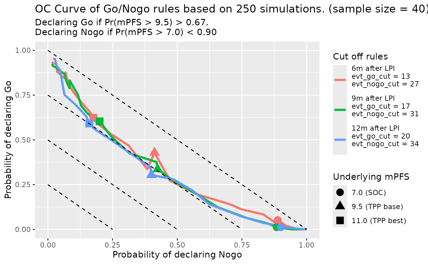
oc_fig_smooth
#> `geom_smooth()` using method = 'loess' and formula = 'y ~ x'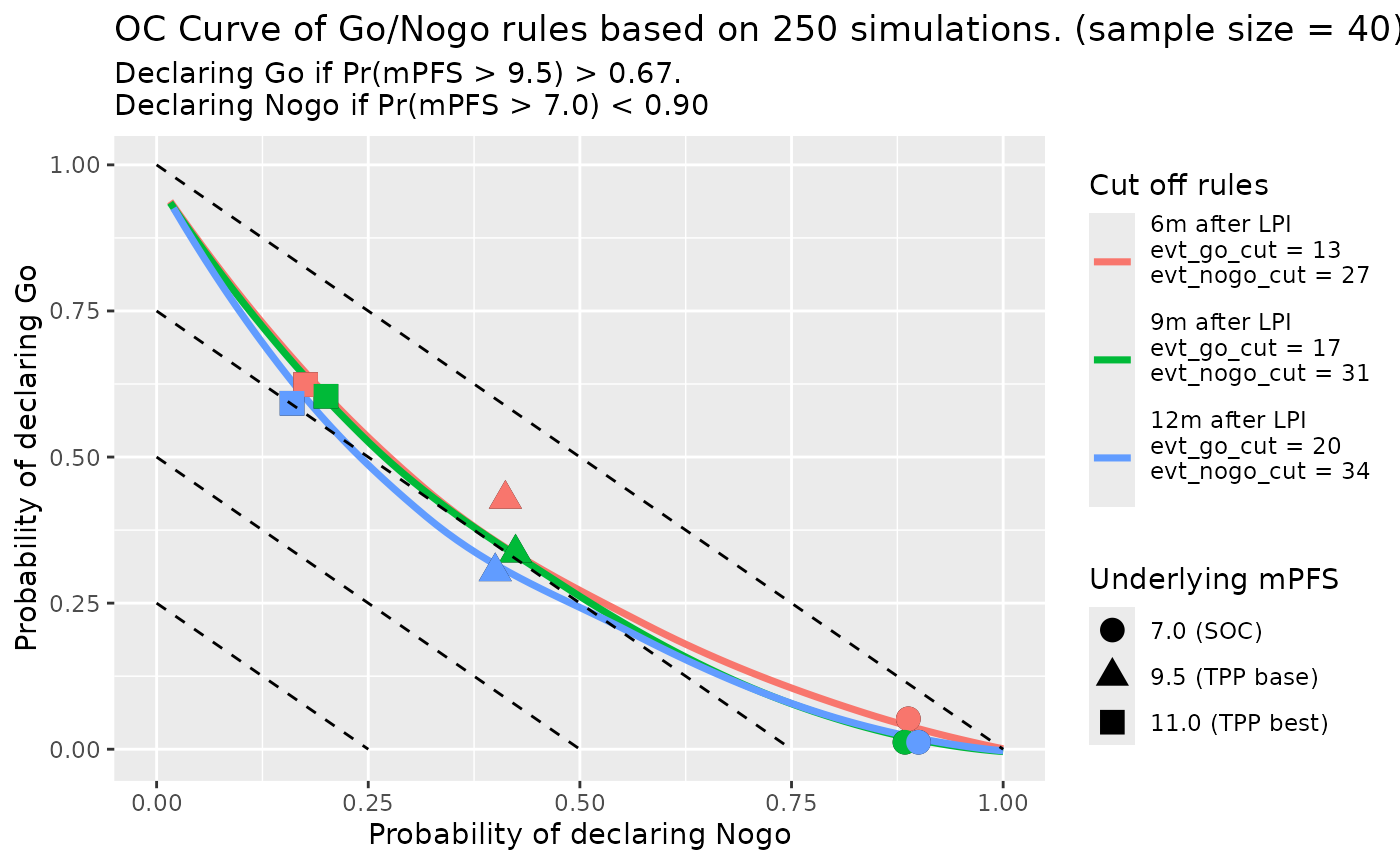
Appendix
Session info
#> ─ Session info ───────────────────────────────────────────────────────────────
#>  setting  value
#>  version  R version 4.4.1 (2024-06-14)
#>  os       Ubuntu 22.04.4 LTS
#>  system   x86_64, linux-gnu
#>  ui       X11
#>  language en
#>  collate  C.UTF-8
#>  ctype    C.UTF-8
#>  tz       UTC
#>  date     2024-06-24
#>  pandoc   3.1.11 @ /opt/hostedtoolcache/pandoc/3.1.11/x64/ (via rmarkdown)
#>
#> ─ Packages ───────────────────────────────────────────────────────────────────
#>  package      * version    date (UTC) lib source
#>  bslib          0.7.0      2024-03-29 [1] RSPM
#>  cachem         1.1.0      2024-05-16 [1] RSPM
#>  cli            3.6.3      2024-06-21 [1] RSPM
#>  codetools      0.2-20     2024-03-31 [3] CRAN (R 4.4.1)
#>  colorspace     2.1-0      2023-01-23 [1] RSPM
#>  cowplot        1.1.3      2024-01-22 [1] RSPM
#>  desc           1.4.3      2023-12-10 [1] RSPM
#>  digest         0.6.35     2024-03-11 [1] RSPM
#>  dplyr        * 1.1.4      2023-11-17 [1] RSPM
#>  evaluate       0.24.0     2024-06-10 [1] RSPM
#>  fansi          1.0.6      2023-12-08 [1] RSPM
#>  farver         2.1.2      2024-05-13 [1] RSPM
#>  fastmap        1.2.0      2024-05-15 [1] RSPM
#>  fs             1.6.4      2024-04-25 [1] RSPM
#>  future       * 1.33.2     2024-03-26 [1] RSPM
#>  future.apply * 1.11.2     2024-03-28 [1] RSPM
#>  generics       0.1.3      2022-07-05 [1] RSPM
#>  ggplot2      * 3.5.1      2024-04-23 [1] RSPM
#>  ggrepel      * 0.9.5      2024-01-10 [1] RSPM
#>  globals        0.16.3     2024-03-08 [1] RSPM
#>  glue           1.7.0      2024-01-09 [1] RSPM
#>  gonogo       * 0.0.0.9024 2024-06-24 [1] local
#>  gtable         0.3.5      2024-04-22 [1] RSPM
#>  highr          0.11       2024-05-26 [1] RSPM
#>  htmltools      0.5.8.1    2024-04-04 [1] RSPM
#>  jquerylib      0.1.4      2021-04-26 [1] RSPM
#>  jsonlite       1.8.8      2023-12-04 [1] RSPM
#>  knitr          1.47       2024-05-29 [1] RSPM
#>  labeling       0.4.3      2023-08-29 [1] RSPM
#>  lattice        0.22-6     2024-03-20 [3] CRAN (R 4.4.1)
#>  lifecycle      1.0.4      2023-11-07 [1] RSPM
#>  listenv        0.9.1      2024-01-29 [1] RSPM
#>  magrittr       2.0.3      2022-03-30 [1] RSPM
#>  Matrix         1.7-0      2024-04-26 [3] CRAN (R 4.4.1)
#>  memoise        2.0.1      2021-11-26 [1] RSPM
#>  mgcv           1.9-1      2023-12-21 [3] CRAN (R 4.4.1)
#>  munsell        0.5.1      2024-04-01 [1] RSPM
#>  nlme           3.1-164    2023-11-27 [3] CRAN (R 4.4.1)
#>  parallelly     1.37.1     2024-02-29 [1] RSPM
#>  pillar         1.9.0      2023-03-22 [1] RSPM
#>  pkgconfig      2.0.3      2019-09-22 [1] RSPM
#>  pkgdown        2.0.9      2024-04-18 [1] any (@2.0.9)
#>  progressr    * 0.14.0     2023-08-10 [1] RSPM
#>  purrr          1.0.2      2023-08-10 [1] RSPM
#>  R6             2.5.1      2021-08-19 [1] RSPM
#>  ragg           1.3.2      2024-05-15 [1] RSPM
#>  Rcpp           1.0.12     2024-01-09 [1] RSPM
#>  rlang          1.1.4      2024-06-04 [1] RSPM
#>  rmarkdown      2.27       2024-05-17 [1] RSPM
#>  sass           0.4.9      2024-03-15 [1] RSPM
#>  scales         1.3.0      2023-11-28 [1] RSPM
#>  sessioninfo    1.2.2      2021-12-06 [1] RSPM
#>  systemfonts    1.1.0      2024-05-15 [1] RSPM
#>  textshaping    0.4.0      2024-05-24 [1] RSPM
#>  tibble         3.2.1      2023-03-20 [1] RSPM
#>  tidyr        * 1.3.1      2024-01-24 [1] RSPM
#>  tidyselect     1.2.1      2024-03-11 [1] RSPM
#>  utf8           1.2.4      2023-10-22 [1] RSPM
#>  vctrs          0.6.5      2023-12-01 [1] RSPM
#>  withr          3.0.0      2024-01-16 [1] RSPM
#>  xfun           0.45       2024-06-16 [1] RSPM
#>  yaml           2.3.8      2023-12-11 [1] RSPM
#>
#>  [1] /home/runner/work/_temp/Library
#>  [2] /opt/R/4.4.1/lib/R/site-library
#>  [3] /opt/R/4.4.1/lib/R/library
#>
#> ──────────────────────────────────────────────────────────────────────────────