BLRM specification
BLRM_specification.RmdNote: In this report, we think all subjects are evaluable!!!
This vignette is about how we setup a BLRM specification document at design stage of a trial. Its content is heavily inspired by Attachment 11 of Tal protocol. This report contains these parts:
Setup the trial information
Prior settings of the BLRM model
Run some hypothetical dose escalation scenarios to see how the model will behave when the data is collected
Simulation under various underlying DLT settings to study the operation characteristics of the BLRM
library(tidyverse)
#> ── Attaching core tidyverse packages ──────────────────────── tidyverse 2.0.0 ──
#> ✔ dplyr     1.1.4     ✔ readr     2.1.5
#> ✔ forcats   1.0.0     ✔ stringr   1.5.1
#> ✔ ggplot2   3.5.1     ✔ tibble    3.2.1
#> ✔ lubridate 1.9.3     ✔ tidyr     1.3.1
#> ✔ purrr     1.0.2
#> ── Conflicts ────────────────────────────────────────── tidyverse_conflicts() ──
#> ✖ dplyr::filter() masks stats::filter()
#> ✖ dplyr::lag()    masks stats::lag()
#> ℹ Use the conflicted package (<http://conflicted.r-lib.org/>) to force all conflicts to become errors
library(crmPack)
#> Registered S3 method overwritten by 'crmPack':
#>   method       from
#>   print.gtable gtable
#> Type crmPackHelp() to open help browser
#> Type crmPackExample() to open example

# for progress report
library(progressr)
handlers("cli")

# for table output
library(flextable)
#>
#> Attaching package: 'flextable'
#>
#> The following object is masked from 'package:purrr':
#>
#>     compose

library(BLRMeval)Prior specification
ref_dose <- 300
prior_dlt_info <- c(0.01, 0.20)    # prior DLT rate guess at `dose_grid[1]` and `ref_dose`
# prior_mean <- c(-0.8472979, -0.8420924)
prior_mean <- Find_AB(dose_vec = c(dose_grid[1], ref_dose),
                      prob_vec = prior_dlt_info,
                      ref_dose = ref_dose,
                      logb = TRUE)
prior_cov <- matrix(c(2 ^ 2, 0, 0, 1 ^ 2), nrow = 2)
# Initialize the CRM model.
initial_model <- LogisticLogNormal(
    mean = prior_mean,
    cov = prior_cov,
    ref_dose = ref_dose
)
dose_vec <- c(0.15, ref_dose)
dlt_rates <- plogis(prior_mean[1] + exp(prior_mean[2]) * log(dose_vec / ref_dose))
The DLT at 0.15ug/kg is 1%.
The DLT at 300ug/kg is 20%.
ft_res <- Flextable_TA(prior_mean, prior_cov)
ft_res
Means |
Standard Deviation |
Correlation |
|---|---|---|
(-1.386, -0.862) |
(2, 1) |
0 |
Summary the prior information
# Fix JAGS sampling seed, because prior samples will be used in later OC simulation settings
prior_mcmc_options <- McmcOptions(burnin = 10000, step = 20, samples = 100000,
                                  rng_kind = "Mersenne-Twister",
                                  rng_seed = prior_summary_seed)

prior_samples <- mcmc(empty_data, model = initial_model, prior_mcmc_options, from_prior = TRUE)

# check table t14-7
res <- sapply(dose_grid,
              Summary_crmPack_Samples,
              ref_dose = initial_model@ref_dose,
              samples = prior_samples, prob_cut = prob_target_cut)

# formatC(t(res), digits = 3, format = "f")
prior_res <- data.frame(dose = dose_grid, t(res))
ft_res <- Flextable_TB(
    prior_res %>% select(-na_num),
    prob_target_cut,
    digits = 3,
    ewoc = ewoc_cut
)
ft_res
Dose |
Probability of DLT in |
Mean |
SD |
Quantiles |
||||
|---|---|---|---|---|---|---|---|---|
[0, 0.16) |
[0.16, 0.3) |
[0.3, 1] |
2.5% |
50% |
97.5% |
|||
0.150 |
0.865 |
0.056 |
0.079 |
0.073 |
0.158 |
0.000 |
0.007 |
0.627 |
0.500 |
0.841 |
0.065 |
0.094 |
0.085 |
0.170 |
0.000 |
0.011 |
0.674 |
1.500 |
0.813 |
0.074 |
0.113 |
0.100 |
0.184 |
0.000 |
0.017 |
0.719 |
5.000 |
0.771 |
0.089 |
0.140 |
0.121 |
0.200 |
0.000 |
0.028 |
0.766 |
15.000 |
0.720 |
0.105 |
0.174 |
0.148 |
0.217 |
0.000 |
0.045 |
0.809 |
50.000 |
0.642 |
0.126 |
0.232 |
0.189 |
0.239 |
0.000 |
0.079 |
0.855 |
150.000 |
0.535 |
0.151 |
0.314 |
0.246 |
0.263 |
0.002 |
0.137 |
0.898 |
300.000 |
0.446 |
0.160 |
0.394 |
0.300 |
0.281 |
0.005 |
0.199 |
0.928 |
600.000 |
0.362 |
0.154 |
0.484 |
0.367 |
0.306 |
0.007 |
0.282 |
0.964 |
900.000 |
0.322 |
0.150 |
0.528 |
0.404 |
0.318 |
0.008 |
0.333 |
0.980 |
*The doses in bold are not recommended as they do not meet EWOC criterion. | ||||||||
Setup detail rules of the trial according to protocol
The MCMC settings:
test_mcmc_options <- McmcOptions(burnin = 10000, step = 20, samples = 10000,
                                 rng_kind = "Mersenne-Twister",
                                 rng_seed = test_scenario_seed)
The EWOC rule:
# Choose the rule for selecting the next dose.
next_best_rule <- NextBestNCRM(
    target = prob_target_cut,
    overdose = c(prob_target_cut[2], 1),
    max_overdose_prob = ewoc_cut
)
The cohort size rule:
# Choose the rule for the cohort size.
cohort_size1 <- CohortSizeRange(
    intervals = c(0, 50),
    cohort_size = c(1, 3)
)
cohort_size2 <- CohortSizeDLT_AT(
    intervals = c(0, 1),
    cohort_size = c(1, 3)
)
cohort_size3 <- CohortSizeConst2(size = 6, max_size = params$max_subj)

cohort_size_rule <- minSize(
    maxSize(cohort_size1, cohort_size2),
    cohort_size3)
Dose increment rule:
# Choose the rule for dose increments.
# rule1: at most increase 1 level compared with last-dose
increment_rule1 <- IncrementsDoseLevels(levels = 1, basis_level = "last")

# # rule2: [0, 20) - at most increse 2-fold, hence 3-fold dose level
# #        [20, Inf) - at most increase 0.5, hence 1.5-fold dose level
# increment_rule2 <- IncrementsRelative(
#     intervals = c(0, 13.5),
#     increments = c(2, 0.5)
# )
#
# # rule3: 0 DLT - at most increase 2-fold, hence 3-fold dose level
# #        >= 1 DLT - at most increase 0.5, hence 1.5-fold dose level
# # NOTE: dose level 4.5, DLT 1, can not increase to dose level 13.5!!!
# #       This is a flaw in protocol!!!
# increment_rule3 <- IncrementsRelativeDLT(
#     intervals = c(0, 1),
#     increments = c(2, 0.5)
# )

increment_rule <- increment_rule1
Trial stopping rule:
# Choose the rule for stopping.
stop_atom1 <- StoppingMinPatients(nPatients = as.integer(params$max_subj),
                                  report_label = paste0("max_subj_", as.integer(params$max_subj)))
stop_atom2 <- StoppingPatientsNearDose(nPatients = as.integer(params$mtd_subj),
                                       percentage = 0,
                                       report_label = paste0("subj_at_mtd_", params$mtd_subj))
stop_atom3 <- StoppingMissingDose(report_label = "NA_recommend")
stop_atom4 <- StoppingTargetProb(target = prob_target_cut, prob = 0.5, report_label = "dlt_prob_target_50%")
stop_atom5 <- StoppingPatientsNearDose(nPatients = 12,
                                       percentage = 0,
                                       report_label = paste0("subj_at_mtdmax_", 12))

stop_mtd <- StoppingAll(stop_list = c(stop_atom2, stop_atom4),
                        report_label = "stop_found_mtd")

stop_mtd_max <- StoppingAny(stop_list = c(stop_mtd, stop_atom5),
                            report_label = "stop_any_mtd")

stop_rule <- StoppingAny(stop_list = c(stop_atom1, stop_mtd_max, stop_atom3),
                         report_label = "stop_any_full")
Summary of the design
Then we can specify the full design:
# Initialize the design.
design <- Design(
    model = initial_model,
    nextBest = next_best_rule,
    stopping = stop_rule,
    increments = increment_rule,
    cohort_size = cohort_size_rule,
    data = empty_data,
    startingDose = dose_grid[1]
)
This following sections summarizing the BLRM design are auto
generated from crmPack’s knit_print(). The
output will mostly work for rendering html output. When rendering
word/pdf output, these auto generated content may be not that user
friendly. If word output is really wanted, one can produce the html
version and open it with Word. Modern versions of Word can handle this
type of html output quite well.
Design
Dose toxicity model
A logistic log normal model will describe the relationship between dose and toxicity: where dref denotes a reference dose.
The prior for θ is given by
The reference dose will be 300.00.
Stopping rule
stop_any_full: If any of the following rules are
TRUE:
max_subj_74: If 74 or more participants have been treated.
-
stop_any_mtd: If either of the following rules are
TRUE:-
stop_found_mtd: If both of the following rules are
TRUE:subj_at_mtd_6: If 6 or more participants have been treated at the next best dose.
dlt_prob_target_50%: If the probability of toxicity at the next best dose is in the range [0.16, 0.30] is at least 0.50.
subj_at_mtdmax_12: If 12 or more participants have been treated at the next best dose.
-
NA_recommend: If the dose returned by
nextBest()isNA, or if the trial includes a placebo dose, the placebo dose.
Escalation rule
The maximum increment between cohorts is 1 level relative to the dose used in the previous cohort.
Dose recommendation
The dose recommended for the next cohort will be chosen in the following way. First, doses that are ineligible according to the increments rule will be discarded. Next, any dose for which the mean posterior probability of toxicity being in the overdose range - (0.3, 1] - is 0.25 or more will also be discarded. Finally, the dose amongst those remaining which has the highest chance that the mean posterior probability of toxicity is in the target toxicity range of 0.16 to 0.3 (inclusive) will be selected.
Cohort size
The minimum of the cohort sizes defined in the following rules:
-
The maximum of the cohort sizes defined in the following rules:
- Defined by the dose to be used in the next cohort
Lower Upper Cohort size 0 50 1 50 Inf 3 - Defined by the number of toxicities so far observed
Note: during the accelerated titration to standard dose escalation transition stage, a cohort size of 2 will be proposed. And the last dose level administrated will be directly recommended as the next dose level ifLower Upper Cohort size 0 1 1 1 Inf 3 NextBestNCRM_AT()is used.
- Defined by the dose to be used in the next cohort
A constant size of 6 participants. Note: if the constant cohort size of 6 for the next reocommended dose will make the total sample size exceeds 74, then the next cohort size will be decreased so that the total sample size is at just 74.
Hypothetical Dose Escalation Scenarios
Now that the model has been established, we can test run the model under various data scenarios to see how it would behave as the trial undergo.
Scenario 1: a quite smooth scenario
First, list the scenarios:
scenario_list <- list(
    s1 = data.frame(
        x = c(0.15),
        y = c(0),
        ID = 1,
        cohort = 1
    ),
    s2 = data.frame(
        x = c(0.15, 0.5),
        y = c(0, 0),
        ID = 1 : 2,
        cohort = 1 : 2
    ),
    s3 = data.frame(
        x = c(0.15, 0.5, 1.5),
        y = c(0, 0, 0),
        ID = 1 : 3,
        cohort = 1 : 3
    ),
    s4 = data.frame(
        x = c(0.15, 0.5, 1.5, 5, 5, 5),
        y = c(0, 0, 0, 0, 0, 0),
        ID = 1 : 6,
        cohort = c(1 : 3, 4, 4, 4)
    ),
    s5 = data.frame(
        x = c(0.15, 0.5, 1.5, 5, 5, 5, 15, 15, 15),
        y = c(0, 0, 0, 0, 0, 0, 0, 0, 0),
        ID = 1 : 9,
        cohort = c(1 : 3, 4, 4, 4, 5, 5, 5)
    ),
    s6 = data.frame(
        x = c(0.15, 0.5, 1.5, 5, 5, 5, 15, 15, 15, 50, 50, 50),
        y = c(0, 0, 0, 0, 0, 0, 0, 0, 0, 1, 0, 0),
        ID = 1 : 12,
        cohort = c(1 : 3, 4, 4, 4, 5, 5, 5, 6, 6, 6)
    ),
    s7 = data.frame(
        x = c(0.15, 0.5, 1.5, 5, 5, 5, 15, 15, 15, 50, 50, 50, 50, 50, 50),
        y = c(0, 0, 0, 0, 0, 0, 0, 0, 0, 1, 0, 0, 0, 0, 0),
        ID = 1 : 15,
        cohort = c(1 : 3, 4, 4, 4, 5, 5, 5, 6, 6, 6, 7, 7, 7)
    ),
    s8 = data.frame(
        x = c(0.15, 0.5, 1.5, 5, 5, 5, 15, 15, 15, 50, 50, 50, 50, 50, 50, 150, 150, 150),
        y = c(0, 0, 0, 0, 0, 0, 0, 0, 0, 1, 0, 0, 0, 0, 0, 0, 0, 0),
        ID = 1 : 18,
        cohort = c(1 : 3, 4, 4, 4, 5, 5, 5, 6, 6, 6, 7, 7, 7, 8, 8, 8)
    )
)
Now we test our design on these scenarios
res <- list()
with_progress({
    p <- progressor(length(scenario_list))
    for(s_idx in seq(length(scenario_list))){
        scenario_data <- scenario_list[[s_idx]]
        cur_res <- Test_Scenario(scenario_data,
                                 dose_grid = dose_grid,
                                 initial_model = initial_model,
                                 increment_rule = increment_rule,
                                 next_best_rule = next_best_rule,
                                 stop_rule = stop_rule,
                                 cohort_size_rule = cohort_size,
                                 mcmc_options = test_mcmc_options) %>%
            mutate(scenario = s_idx, .before = everything())
        res[[s_idx]] <- cur_res
        p(message = c("Scenario ", s_idx, " finished!"))
    }
})
table_c <- bind_rows(!!!res) %>%
    mutate(cohort_id = as.integer(cohort_id),
           treated = as.integer(treated),
           with_dlt = as.integer(with_dlt))
ft_res <- Flextable_TC(table_c, digits = 4, dose_unit = dose_unit)
ft_res
Scenario |
Cohort ID |
Dose (ug/kg) |
N |
Number of DLT |
Recommended Next Dose |
P(Target) |
P(Over) |
Median P(d) |
|---|---|---|---|---|---|---|---|---|
1 |
1 |
0.1500 |
1 |
0 |
0.5000 |
0.0525 |
0.0493 |
0.0077 |
2 |
1 |
0.1500 |
1 |
0 |
||||
2 |
0.5000 |
1 |
0 |
1.5000 |
0.0607 |
0.0417 |
0.0101 |
|
3 |
1 |
0.1500 |
1 |
0 |
||||
2 |
0.5000 |
1 |
0 |
|||||
3 |
1.5000 |
1 |
0 |
5.0000 |
0.0721 |
0.0407 |
0.0153 |
|
4 |
1 |
0.1500 |
1 |
0 |
||||
2 |
0.5000 |
1 |
0 |
|||||
3 |
1.5000 |
1 |
0 |
|||||
4 |
5.0000 |
3 |
0 |
15.0000 |
0.0607 |
0.0239 |
0.0180 |
|
5 |
1 |
0.1500 |
1 |
0 |
||||
2 |
0.5000 |
1 |
0 |
|||||
3 |
1.5000 |
1 |
0 |
|||||
4 |
5.0000 |
3 |
0 |
|||||
5 |
15.0000 |
3 |
0 |
50.0000 |
0.0764 |
0.0302 |
0.0275 |
|
6 |
1 |
0.1500 |
1 |
0 |
||||
2 |
0.5000 |
1 |
0 |
|||||
3 |
1.5000 |
1 |
0 |
|||||
4 |
5.0000 |
3 |
0 |
|||||
5 |
15.0000 |
3 |
0 |
|||||
6 |
50.0000 |
3 |
1 |
50.0000 |
0.2413 |
0.0983 |
0.1109 |
|
7 |
1 |
0.1500 |
1 |
0 |
||||
2 |
0.5000 |
1 |
0 |
|||||
3 |
1.5000 |
1 |
0 |
|||||
4 |
5.0000 |
3 |
0 |
|||||
5 |
15.0000 |
3 |
0 |
|||||
6 |
50.0000 |
3 |
1 |
|||||
7 |
50.0000 |
3 |
0 |
150.0000 |
0.2609 |
0.1857 |
0.1418 |
|
8 |
1 |
0.1500 |
1 |
0 |
||||
2 |
0.5000 |
1 |
0 |
|||||
3 |
1.5000 |
1 |
0 |
|||||
4 |
5.0000 |
3 |
0 |
|||||
5 |
15.0000 |
3 |
0 |
|||||
6 |
50.0000 |
3 |
1 |
|||||
7 |
50.0000 |
3 |
0 |
|||||
8 |
150.0000 |
3 |
0 |
300.0000 |
0.2472 |
0.1647 |
0.1315 |
Scenario 2: one with higher occurrence of DLT
First, list the scenarios:
scenario_list <- list(
    s1 = data.frame(
        x = c(0.15),
        y = c(0),
        ID = 1,
        cohort = 1
    ),
    s2 = data.frame(
        x = c(0.15, 0.5),
        y = c(0, 0),
        ID = 1 : 2,
        cohort = 1 : 2
    ),
    s3 = data.frame(
        x = c(0.15, 0.5, 1.5, 1.5, 1.5),
        y = c(0, 0, 1, 0, 0),
        ID = 1 : 5,
        cohort = c(1, 2, 3, 3, 3)
    ),
    s4 = data.frame(
        x = c(0.15, 0.5, 1.5, 1.5, 1.5, 1.5, 1.5, 1.5),
        y = c(0, 0, 1, 0, 0, 0, 0, 0),
        ID = 1 : 8,
        cohort = c(1, 2, 3, 3, 3, 4, 4, 4)
    ),
    s5 = data.frame(
        x = c(0.15, 0.5, 1.5, 1.5, 1.5, 1.5, 1.5, 1.5, 5, 5, 5),
        y = c(0, 0, 1, 0, 0, 0, 0, 0, 0, 0, 0),
        ID = 1 : 11,
        cohort = c(1, 2, 3, 3, 3, 4, 4, 4, 5, 5, 5)
    ),
    s6 = data.frame(
        x = c(0.15, 0.5, 1.5, 1.5, 1.5, 1.5, 1.5, 1.5, 5, 5, 5, 15, 15, 15),
        y = c(0, 0, 1, 0, 0, 0, 0, 0, 0, 0, 0, 1, 0, 0),
        ID = 1 : 14,
        cohort = c(1, 2, 3, 3, 3, 4, 4, 4, 5, 5, 5, 6, 6, 6)
    ),
    s7 = data.frame(
        x = c(0.15, 0.5, 1.5, 1.5, 1.5, 1.5, 1.5, 1.5, 5, 5, 5, 15, 15, 15, 15, 15, 15),
        y = c(0, 0, 1, 0, 0, 0, 0, 0, 0, 0, 0, 1, 0, 0, 1, 0, 0),
        ID = 1 : 17,
        cohort = c(1, 2, 3, 3, 3, 4, 4, 4, 5, 5, 5, 6, 6, 6, 7, 7, 7)
    ),
    s8 = data.frame(
        x = c(0.15, 0.5, 1.5, 1.5, 1.5, 1.5, 1.5, 1.5, 5, 5, 5, 15, 15, 15, 15, 15, 15, 15, 15, 15),
        y = c(0, 0, 1, 0, 0, 0, 0, 0, 0, 0, 0, 1, 0, 0, 1, 0, 0, 1, 1, 0),
        ID = 1 : 20,
        cohort = c(1, 2, 3, 3, 3, 4, 4, 4, 5, 5, 5, 6, 6, 6, 7, 7, 7, 8, 8, 8)
    )
)
Now we test our design on these scenarios
res <- list()
with_progress({
    p <- progressor(length(scenario_list))
    for(s_idx in seq(length(scenario_list))){
        scenario_data <- scenario_list[[s_idx]]
        cur_res <- Test_Scenario(scenario_data,
                                 dose_grid = dose_grid,
                                 initial_model = initial_model,
                                 increment_rule = increment_rule,
                                 next_best_rule = next_best_rule,
                                 stop_rule = stop_rule,
                                 cohort_size_rule = cohort_size,
                                 mcmc_options = test_mcmc_options) %>%
            mutate(scenario = s_idx, .before = everything())
        res[[s_idx]] <- cur_res
        p(message = c("Scenario ", s_idx, " finished!"))
    }
})
table_c <- bind_rows(!!!res) %>%
    mutate(cohort_id = as.integer(cohort_id),
           treated = as.integer(treated),
           with_dlt = as.integer(with_dlt))
ft_res <- Flextable_TC(table_c, digits = 4, dose_unit = dose_unit)
ft_res
Scenario |
Cohort ID |
Dose (ug/kg) |
N |
Number of DLT |
Recommended Next Dose |
P(Target) |
P(Over) |
Median P(d) |
|---|---|---|---|---|---|---|---|---|
1 |
1 |
0.1500 |
1 |
0 |
0.5000 |
0.0525 |
0.0493 |
0.0077 |
2 |
1 |
0.1500 |
1 |
0 |
||||
2 |
0.5000 |
1 |
0 |
1.5000 |
0.0607 |
0.0417 |
0.0101 |
|
3 |
1 |
0.1500 |
1 |
0 |
||||
2 |
0.5000 |
1 |
0 |
|||||
3 |
1.5000 |
3 |
1 |
1.5000 |
0.2422 |
0.1640 |
0.1274 |
|
4 |
1 |
0.1500 |
1 |
0 |
||||
2 |
0.5000 |
1 |
0 |
|||||
3 |
1.5000 |
3 |
1 |
|||||
4 |
1.5000 |
3 |
0 |
5.0000 |
0.2566 |
0.1225 |
0.1194 |
|
5 |
1 |
0.1500 |
1 |
0 |
||||
2 |
0.5000 |
1 |
0 |
|||||
3 |
1.5000 |
3 |
1 |
|||||
4 |
1.5000 |
3 |
0 |
|||||
5 |
5.0000 |
3 |
0 |
15.0000 |
0.2542 |
0.1051 |
0.1165 |
|
6 |
1 |
0.1500 |
1 |
0 |
||||
2 |
0.5000 |
1 |
0 |
|||||
3 |
1.5000 |
3 |
1 |
|||||
4 |
1.5000 |
3 |
0 |
|||||
5 |
5.0000 |
3 |
0 |
|||||
6 |
15.0000 |
3 |
1 |
15.0000 |
0.3775 |
0.1767 |
0.1751 |
|
7 |
1 |
0.1500 |
1 |
0 |
||||
2 |
0.5000 |
1 |
0 |
|||||
3 |
1.5000 |
3 |
1 |
|||||
4 |
1.5000 |
3 |
0 |
|||||
5 |
5.0000 |
3 |
0 |
|||||
6 |
15.0000 |
3 |
1 |
|||||
7 |
15.0000 |
3 |
1 |
15.0000 |
0.4567 |
0.2291 |
0.2077 |
|
8 |
1 |
0.1500 |
1 |
0 |
||||
2 |
0.5000 |
1 |
0 |
|||||
3 |
1.5000 |
3 |
1 |
|||||
4 |
1.5000 |
3 |
0 |
|||||
5 |
5.0000 |
3 |
0 |
|||||
6 |
15.0000 |
3 |
1 |
|||||
7 |
15.0000 |
3 |
1 |
|||||
8 |
15.0000 |
3 |
2 |
5.0000 |
0.5382 |
0.1988 |
0.2155 |
Operating Characteristics
Preparation
First we specify the hypothetical DLT scenarios
dlt_settings_list <- data.frame(
    s1 = prior_res$p50,
    s2 = prior_res$p50 * 1.5,
    s3 = prior_res$p50 * 0.5,
    s4 = c(0.100, 0.150, 0.200, 0.250, 0.300, 0.350, 0.400, 0.450, 0.500, 0.550),
    s5 = c(0.010, 0.030, 0.050, 0.070, 0.095, 0.120, 0.150, 0.190, 0.230, 0.280),
    s6 = c(0.250, 0.300, 0.350, 0.400, 0.450, 0.500, 0.550, 0.600, 0.650, 0.700)
)
# print(dlt_settings_list)
f1 <- data.frame(dose = dose_grid, dlt_settings_list) %>%
    pivot_longer(cols = starts_with("s"),
                 names_to = "dlt_setting",
                 values_to = "dlt_rate") %>%
    mutate(`DLT Scenario` = LETTERS[as.integer(str_sub(dlt_setting, start = 2, end = -1))]) %>%
    ggplot(aes(x = dose, y = dlt_rate, color = `DLT Scenario`)) +
    geom_line() +
    geom_point() +
    geom_hline(yintercept = prob_target_cut, linetype = "dashed") +
    labs(x = paste0("Dose (", dose_unit, ")"), y = "DLT Rate")

f2 <- f1 +
    scale_x_log10(labels = function(breaks) formatC(breaks, format = "fg"))

cowplot::plot_grid(f1, f2, ncol = 1, align = "hv")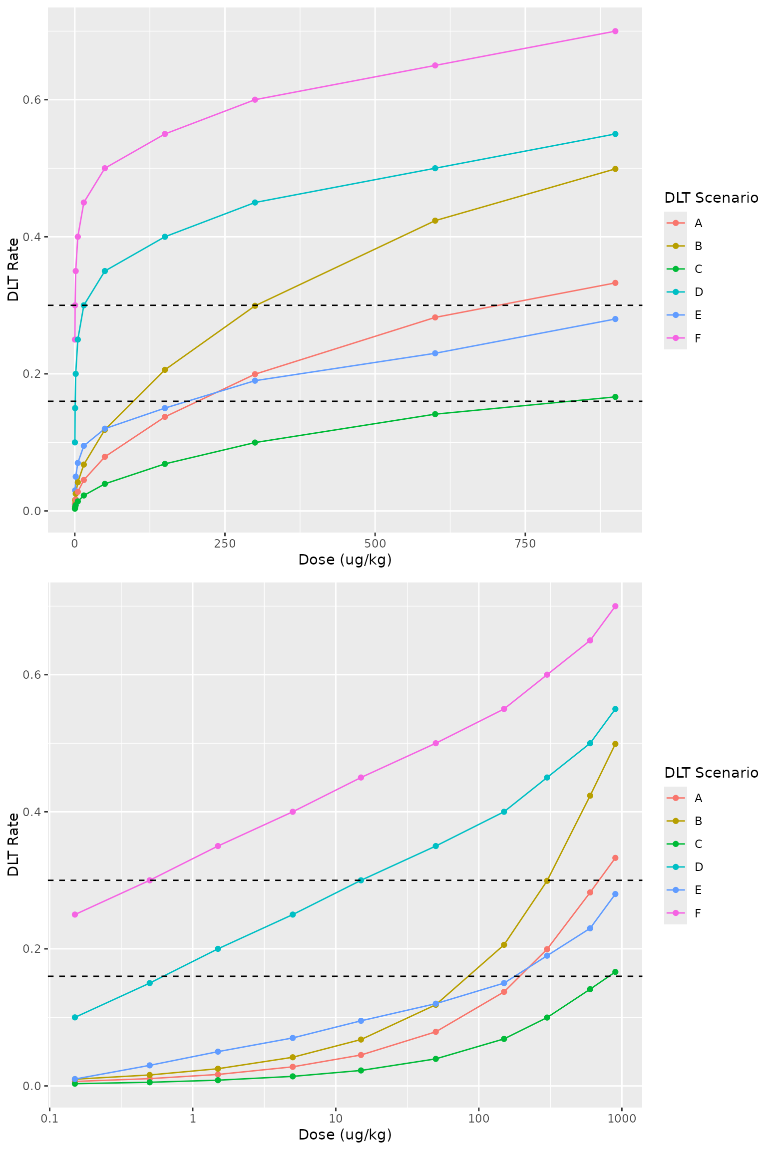
ft_res <- Flextable_TD(dose_grid, dlt_settings_list, prob_target_cut, digits = 4, dose_unit = dose_unit)
ft_res
Scenario |
A |
B |
C |
D |
E |
F |
|---|---|---|---|---|---|---|
Dose (ug/kg) |
P(DLT) |
|||||
0.150 |
0.007 |
0.010 |
0.003 |
0.100 |
0.010 |
0.250 |
0.500 |
0.011 |
0.016 |
0.005 |
0.150 |
0.030 |
0.300 |
1.500 |
0.017 |
0.025 |
0.008 |
0.200 |
0.050 |
0.350 |
5.000 |
0.028 |
0.042 |
0.014 |
0.250 |
0.070 |
0.400 |
15.000 |
0.045 |
0.068 |
0.023 |
0.300 |
0.095 |
0.450 |
50.000 |
0.079 |
0.118 |
0.039 |
0.350 |
0.120 |
0.500 |
150.000 |
0.137 |
0.206 |
0.069 |
0.400 |
0.150 |
0.550 |
300.000 |
0.199 |
0.299 |
0.100 |
0.450 |
0.190 |
0.600 |
600.000 |
0.282 |
0.424 |
0.141 |
0.500 |
0.230 |
0.650 |
900.000 |
0.333 |
0.499 |
0.166 |
0.550 |
0.280 |
0.700 |
Bolded doses are with true P(DLT) within the target toxicity interval [16.00%, 30.00%). | ||||||
Note: Next we adjust the design, because the full design in simulation is different from previous
# check different back-up plan whan `NA` dose is recommended
# This typically means the model thinks all doses are too toxic
# 0 -- No back up plan, stop the trial
# 1 -- Use the 1st dose in dose grid as back up and start to escalation again
na_method_vec <- c(0L, 1L)
oc_cohort_size_rule <- CohortSizeConst(3)   # cohort size fixed at 3 when OC simulation
Next are some settings for simulation
RNGkind("L'Ecuyer-CMRG")    # parallel-safe RNG kind. If you want to use parallel simulation, this is necessary
nsim <- 50    # number of simulations
seed <- 1234    # seed for R side
res_folder <- params$res_folder
use_parallel <- TRUE
ncores <- 10    # number of cores
oc_mcmc_options <- McmcOptions(burnin = 10, step = 2, samples = 50,
                               rng_kind = "Mersenne-Twister",
                               rng_seed = oc_simulation_seed)
previous_idx <- 0    # A hotfix for controlling the starting DLT setting for OC simulation
                     # only settings with `dlt_setting_idx > previous_idx` will
                     # actual run the simulation
Note: To simplify the computation, the MCMC settings
for the simulation in this vignette is setup in a unreasonable low value
(burnin = 10, step = 2,
samples = 50). Please adjust it according to your needs in
real world application.
Note: For parallel simulation, crmPack
will internally use the minimum between ncores you set and
parallelly::availableCores() to make sure you don’t
accidentally overwhelm the machine. So, even we set
ncores = 10 previously, when rendering this vignette, only
2 core(s) is/are used.
Note: For perfect replica of the results, we have to control the random seeds, even across different parallel cores, on both R and JAGS sides:
The JAGS seed is controlled via
McmcOptions(). By setting this seed, same observed data and same toxicity model will give the exactly same estimated toxicity curve, even they are at different simulations. This means there will be no MCMC randomness across multiple runs of the same simulation. The estimated toxicity of the dose levels will be the same as long as given same observed data and model.For R seed, it’s recommended to use the
seedparameter insimulate()call. In this way, it is not necessary to set the parallel-safe “L’Ecuyer-CMRG” seed kind in the R environment, even in parallel simulations. That’s becausecrmPackwill take care of the random seed setting even under parallel simulation settings. Though its implementation is the topic of another discussion.
Carry out simulation
Now we carry out the full simulation
for(na_method_idx in seq_along(na_method_vec)){
    scenario_summary <- list()
    scenario_summary_ssg <- list()
    for(dlt_setting_idx in seq_along(dlt_settings_list)){
        if(dlt_setting_idx > previous_idx){
            # print(paste0("DLT setting - ", dlt_setting_idx,
            #              " Start!"))
            na_method <- na_method_vec[na_method_idx]
            dlt_setting <- dlt_settings_list[[dlt_setting_idx]]

            # define/expand the true dlt rate function
            mytruth <- function(dose){
                x <- dose_grid
                y <- dlt_setting
                res <- approx(x = x, y = y, xout = dose, method = "linear")
                res$y
            }

            oc_next_best_rule <- NextBestNCRM_AT(
                target = prob_target_cut,
                overdose = c(prob_target_cut[2], 1),
                max_overdose_prob = ewoc_cut,
                na_method = na_method)

            oc_design <- Design(
                model = initial_model,
                nextBest = oc_next_best_rule,
                stopping = stop_rule,
                increments = increment_rule1,    # fixed level increment
                cohort_size = oc_cohort_size_rule,
                data = empty_data,
                startingDose = dose_grid[1]
            )

            time <- system.time(my_sims <- simulate(oc_design,
                                                    args = NULL,
                                                    truth = mytruth,
                                                    nsim = nsim,
                                                    seed = seed,
                                                    mcmcOptions = oc_mcmc_options,
                                                    parallel = use_parallel,
                                                    nCores = ncores
            ))

            # crmPack summary
            sim_sum <- summary(my_sims, mytruth, target = prob_target_cut)

            # my dose level summary
            my_summary1 <- My_Summary_Dose_Level(my_sims, sim_sum, mytruth,
                                                 oc_design, oc_mcmc_options,
                                                 progress_interval = 10)
            # my scenario level summary
            my_summary2 <- My_Summary_Scenario_Level2(my_sims, mytruth,
                                                     oc_design, oc_mcmc_options)

            # filter out the simulations that fail to make dose recommendation
            #   and then summary the remaining simulations
            my_sims_ssg <- my_sims

            ssg_filter_out_idx <- rep(FALSE, nsim)
            for(sim_idx in seq(nsim)){
                sim_max_subj <- max(my_sims@data[[sim_idx]]@ID)
                sim_na_recommend <- is.na(my_sims@doses[sim_idx])
                # if(sim_max_subj < 18)  ssg_filter_out_idx[sim_idx] <- TRUE
                if(sim_na_recommend)  ssg_filter_out_idx[sim_idx] <- TRUE
            }
            ssg_filter_out_idx <- (1 : nsim)[ssg_filter_out_idx]
            if(length(ssg_filter_out_idx) > 0){
                my_sims_ssg@fit[ssg_filter_out_idx] <- NULL
                my_sims_ssg@stop_report <- my_sims_ssg@stop_report[-ssg_filter_out_idx, , drop = FALSE]
                my_sims_ssg@stop_reasons[ssg_filter_out_idx] <- NULL
                my_sims_ssg@additional_stats[ssg_filter_out_idx] <- NULL
                my_sims_ssg@data[ssg_filter_out_idx] <- NULL
                my_sims_ssg@doses <- my_sims_ssg@doses[-ssg_filter_out_idx]
            }


            my_summary2_ssg <- My_Summary_Scenario_Level2(my_sims_ssg, mytruth,
                                                         oc_design, oc_mcmc_options)

            scenario_summary[[dlt_setting_idx]] <- bind_cols(
                tibble(scenario_idx = LETTERS[dlt_setting_idx]),
                my_summary2
            )

            scenario_summary_ssg[[dlt_setting_idx]] <- bind_cols(
                tibble(scenario_idx = LETTERS[dlt_setting_idx]),
                my_summary2_ssg
            )

            # --- print progress info and save results---
            if(params$save_res){
                file_name <- paste0("DLT_setting_", dlt_setting_idx,
                                "_namethod_", na_method,
                                ".rds")
                saveRDS(list(sim_data = my_sims,
                             true_fun = mytruth,
                             sim_summary = sim_sum,
                             my_sim_sum1 = my_summary1,
                             my_sim_sum2 = my_summary2,
                             my_sim_sum2_ssg = my_summary2_ssg,
                             design = oc_design,
                             mcmcoptions = oc_mcmc_options),
                        file = paste0(res_folder, file_name))

                file_name_fig1 <- paste0(xfun::sans_ext(file_name), "_1.pdf")
                file_name_fig2 <- paste0(xfun::sans_ext(file_name), "_2.pdf")

                cairo_pdf(filename = paste0(res_folder, file_name_fig1))
                print(plot(plot(my_sims)))
                dev.off()

                cairo_pdf(filename = paste0(res_folder, file_name_fig2))
                print(plot(plot(sim_sum)))
                dev.off()

                file_name_report <- paste0(xfun::sans_ext(file_name), "_summary.txt")

                cat(paste0("DLT setting - ", dlt_setting_idx,
                           " Finished!\n"),
                    file = paste0(res_folder, file_name_report), append = FALSE, sep = "\n")
                capture.output(x = print(time), file = paste0(res_folder, file_name_report), append = TRUE)

                cat("",file = paste0(res_folder, file_name_report), append = TRUE, sep = "\n")
                cat("crmPack summary: ",file = paste0(res_folder, file_name_report), append = TRUE, sep = "\n")
                capture.output(x = sim_sum, file = paste0(res_folder, file_name_report), append = TRUE)

                cat("",file = paste0(res_folder, file_name_report), append = TRUE, sep = "\n")
                cat("Dose level summary: ",file = paste0(res_folder, file_name_report), append = TRUE, sep = "\n")
                capture.output(x = print(my_summary1, width = 400), file = paste0(res_folder, file_name_report), append = TRUE)

                cat("",file = paste0(res_folder, file_name_report), append = TRUE, sep = "\n")
                cat("Scenario level summary: ",file = paste0(res_folder, file_name_report), append = TRUE, sep = "\n")
                capture.output(x = print(my_summary2, width = 400), file = paste0(res_folder, file_name_report), append = TRUE)

                cat("",file = paste0(res_folder, file_name_report), append = TRUE, sep = "\n")
                cat("Scenario level summary (SSG): ",file = paste0(res_folder, file_name_report), append = TRUE, sep = "\n")
                capture.output(x = print(my_summary2_ssg, width = 400), file = paste0(res_folder, file_name_report), append = TRUE)

                cat("",file = paste0(res_folder, file_name_report), append = TRUE, sep = "\n")
                cat("Session info: ",file = paste0(res_folder, file_name_report), append = TRUE, sep = "\n")
                capture.output(x = print(sessionInfo(), width = 100), file = paste0(res_folder, file_name_report), append = TRUE)
            }
        }
    }

    cat(paste0("### Summary during simulation", ": \n\n<!-- -->\n\n"))

    cat(paste0("na_method = ", na_method, ": \n\n<!-- -->\n\n"))

    cat(paste0("All simulations", ": \n\n<!-- -->\n\n"))

    cat('\n\n<!-- -->\n\n')

    table_e <- bind_rows(!!!scenario_summary)
    ft_res <- Flextable_TE2(table_e, prob_target_cut, digits = 3)
    flextable::flextable_to_rmd(ft_res)

    cat('\n\n<!-- -->\n\n')

    cat('\n\n<!-- -->\n\n')

    cat(paste0("Filtered simulations that have make final dose recommendations", ": \n\n<!-- -->\n\n"))

    cat('\n\n<!-- -->\n\n')

    table_e2 <- bind_rows(!!!scenario_summary_ssg)
    ft_res <- Flextable_TE2(table_e2, prob_target_cut, digits = 3)
    flextable::flextable_to_rmd(ft_res)
    cat('\n\n<!-- -->\n\n')
}
Summary during simulation:
na_method = 0:
All simulations:
Scenario |
#Sim |
Probability of recommending |
Average proportion |
Average number |
||||||
|---|---|---|---|---|---|---|---|---|---|---|
Dose |
[0, 0.16) |
[0.16, 0.3) |
[0.3, 1] |
A Target |
Dose with |
Per Study |
Experiencing |
in dose level that |
||
A |
50 |
0.000 |
0.440 |
0.420 |
0.140 |
0.221 |
0.052 |
38.580 |
4.060 |
11.040 |
B |
50 |
0.020 |
0.280 |
0.680 |
0.020 |
0.329 |
0.037 |
35.760 |
4.280 |
10.380 |
C |
50 |
0.000 |
0.460 |
0.540 |
0.000 |
0.170 |
0.000 |
42.480 |
3.120 |
11.220 |
D |
50 |
0.320 |
0.040 |
0.320 |
0.320 |
0.329 |
0.152 |
16.440 |
3.300 |
6.240 |
E |
50 |
0.020 |
0.480 |
0.500 |
0.000 |
0.247 |
0.000 |
37.740 |
4.100 |
10.740 |
F |
50 |
0.720 |
0.000 |
0.020 |
0.260 |
0.648 |
0.352 |
8.760 |
2.660 |
4.140 |
Filtered simulations that have make final dose recommendations:
Scenario |
#Sim |
Probability of recommending |
Average proportion |
Average number |
||||||
|---|---|---|---|---|---|---|---|---|---|---|
Dose |
[0, 0.16) |
[0.16, 0.3) |
[0.3, 1] |
A Target |
Dose with |
Per Study |
Experiencing |
in dose level that |
||
A |
50 |
0.000 |
0.440 |
0.420 |
0.140 |
0.221 |
0.052 |
38.580 |
4.060 |
11.040 |
B |
49 |
0.000 |
0.286 |
0.694 |
0.020 |
0.336 |
0.038 |
36.429 |
4.347 |
10.531 |
C |
50 |
0.000 |
0.460 |
0.540 |
0.000 |
0.170 |
0.000 |
42.480 |
3.120 |
11.220 |
D |
34 |
0.000 |
0.059 |
0.471 |
0.471 |
0.474 |
0.223 |
22.235 |
4.176 |
7.765 |
E |
49 |
0.000 |
0.490 |
0.510 |
0.000 |
0.252 |
0.000 |
38.449 |
4.163 |
10.898 |
F |
14 |
0.000 |
0.000 |
0.071 |
0.929 |
0.190 |
0.810 |
18.429 |
4.929 |
6.429 |
Summary during simulation:
na_method = 1:
All simulations:
Scenario |
#Sim |
Probability of recommending |
Average proportion |
Average number |
||||||
|---|---|---|---|---|---|---|---|---|---|---|
Dose |
[0, 0.16) |
[0.16, 0.3) |
[0.3, 1] |
A Target |
Dose with |
Per Study |
Experiencing |
in dose level that |
||
A |
50 |
0.000 |
0.440 |
0.420 |
0.140 |
0.221 |
0.052 |
38.580 |
4.060 |
11.040 |
B |
50 |
0.000 |
0.300 |
0.680 |
0.020 |
0.329 |
0.037 |
36.480 |
4.380 |
10.500 |
C |
50 |
0.000 |
0.460 |
0.540 |
0.000 |
0.170 |
0.000 |
42.480 |
3.120 |
11.220 |
D |
50 |
0.000 |
0.200 |
0.380 |
0.420 |
0.389 |
0.179 |
22.140 |
4.220 |
8.040 |
E |
50 |
0.000 |
0.500 |
0.500 |
0.000 |
0.247 |
0.000 |
38.460 |
4.200 |
10.860 |
F |
50 |
0.000 |
0.000 |
0.620 |
0.380 |
0.592 |
0.408 |
14.460 |
4.400 |
7.920 |
Filtered simulations that have make final dose recommendations:
Scenario |
#Sim |
Probability of recommending |
Average proportion |
Average number |
||||||
|---|---|---|---|---|---|---|---|---|---|---|
Dose |
[0, 0.16) |
[0.16, 0.3) |
[0.3, 1] |
A Target |
Dose with |
Per Study |
Experiencing |
in dose level that |
||
A |
50 |
0.000 |
0.440 |
0.420 |
0.140 |
0.221 |
0.052 |
38.580 |
4.060 |
11.040 |
B |
50 |
0.000 |
0.300 |
0.680 |
0.020 |
0.329 |
0.037 |
36.480 |
4.380 |
10.500 |
C |
50 |
0.000 |
0.460 |
0.540 |
0.000 |
0.170 |
0.000 |
42.480 |
3.120 |
11.220 |
D |
50 |
0.000 |
0.200 |
0.380 |
0.420 |
0.389 |
0.179 |
22.140 |
4.220 |
8.040 |
E |
50 |
0.000 |
0.500 |
0.500 |
0.000 |
0.247 |
0.000 |
38.460 |
4.200 |
10.860 |
F |
50 |
0.000 |
0.000 |
0.620 |
0.380 |
0.592 |
0.408 |
14.460 |
4.400 |
7.920 |
Appendix
Session info
#> ─ Session info ───────────────────────────────────────────────────────────────
#>  setting  value
#>  version  R version 4.4.1 (2024-06-14)
#>  os       Ubuntu 22.04.4 LTS
#>  system   x86_64, linux-gnu
#>  ui       X11
#>  language en
#>  collate  C.UTF-8
#>  ctype    C.UTF-8
#>  tz       UTC
#>  date     2024-08-06
#>  pandoc   3.1.11 @ /opt/hostedtoolcache/pandoc/3.1.11/x64/ (via rmarkdown)
#>
#> ─ Packages ───────────────────────────────────────────────────────────────────
#>  package           * version    date (UTC) lib source
#>  askpass             1.2.0      2023-09-03 [1] RSPM
#>  backports           1.5.0      2024-05-23 [1] RSPM
#>  BLRMeval          * 0.0.0.9005 2024-08-06 [1] local
#>  bslib               0.8.0      2024-07-29 [1] RSPM
#>  cachem              1.1.0      2024-05-16 [1] RSPM
#>  checkmate           2.3.2      2024-07-29 [1] RSPM
#>  cli                 3.6.3      2024-06-21 [1] RSPM
#>  coda                0.19-4.1   2024-01-31 [1] RSPM
#>  colorspace          2.1-1      2024-07-26 [1] RSPM
#>  cowplot             1.1.3      2024-01-22 [1] RSPM
#>  crayon              1.5.3      2024-06-20 [1] RSPM
#>  crmPack           * 2.0.0.9158 2024-08-05 [1] Github (openpharma/crmPack@75659a9)
#>  crul                1.5.0      2024-07-19 [1] RSPM
#>  curl                5.2.1      2024-03-01 [1] RSPM
#>  data.table          1.15.4     2024-03-30 [1] RSPM
#>  desc                1.4.3      2023-12-10 [1] RSPM
#>  digest              0.6.36     2024-06-23 [1] RSPM
#>  dplyr             * 1.1.4      2023-11-17 [1] RSPM
#>  evaluate            0.24.0     2024-06-10 [1] RSPM
#>  fansi               1.0.6      2023-12-08 [1] RSPM
#>  farver              2.1.2      2024-05-13 [1] RSPM
#>  fastmap             1.2.0      2024-05-15 [1] RSPM
#>  flextable         * 0.9.6      2024-05-05 [1] RSPM
#>  fontBitstreamVera   0.1.1      2017-02-01 [1] RSPM
#>  fontLiberation      0.1.0      2016-10-15 [1] RSPM
#>  fontquiver          0.2.1      2017-02-01 [1] RSPM
#>  forcats           * 1.0.0      2023-01-29 [1] RSPM
#>  formatR             1.14       2023-01-17 [1] RSPM
#>  fs                  1.6.4      2024-04-25 [1] RSPM
#>  futile.logger       1.4.3      2016-07-10 [1] RSPM
#>  futile.options      1.0.1      2018-04-20 [1] RSPM
#>  gdtools             0.3.7      2024-03-05 [1] RSPM
#>  generics            0.1.3      2022-07-05 [1] RSPM
#>  GenSA               1.1.14     2024-01-22 [1] RSPM
#>  gfonts              0.2.0      2023-01-08 [1] RSPM
#>  ggplot2           * 3.5.1      2024-04-23 [1] RSPM
#>  glue                1.7.0      2024-01-09 [1] RSPM
#>  gridExtra           2.3        2017-09-09 [1] RSPM
#>  gtable              0.3.5      2024-04-22 [1] RSPM
#>  highr               0.11       2024-05-26 [1] RSPM
#>  hms                 1.1.3      2023-03-21 [1] RSPM
#>  htmltools           0.5.8.1    2024-04-04 [1] RSPM
#>  htmlwidgets         1.6.4      2023-12-06 [1] RSPM
#>  httpcode            0.3.0      2020-04-10 [1] RSPM
#>  httpuv              1.6.15     2024-03-26 [1] RSPM
#>  jquerylib           0.1.4      2021-04-26 [1] RSPM
#>  jsonlite            1.8.8      2023-12-04 [1] RSPM
#>  kableExtra          1.4.0      2024-01-24 [1] RSPM
#>  knitr               1.48       2024-07-07 [1] RSPM
#>  labeling            0.4.3      2023-08-29 [1] RSPM
#>  lambda.r            1.2.4      2019-09-18 [1] RSPM
#>  later               1.3.2      2023-12-06 [1] RSPM
#>  lattice             0.22-6     2024-03-20 [3] CRAN (R 4.4.1)
#>  lifecycle           1.0.4      2023-11-07 [1] RSPM
#>  lubridate         * 1.9.3      2023-09-27 [1] RSPM
#>  magrittr            2.0.3      2022-03-30 [1] RSPM
#>  mime                0.12       2021-09-28 [1] RSPM
#>  munsell             0.5.1      2024-04-01 [1] RSPM
#>  mvtnorm             1.2-5      2024-05-21 [1] RSPM
#>  officer             0.6.6      2024-05-05 [1] RSPM
#>  openssl             2.2.0      2024-05-16 [1] RSPM
#>  parallelly          1.38.0     2024-07-27 [1] RSPM
#>  pillar              1.9.0      2023-03-22 [1] RSPM
#>  pkgconfig           2.0.3      2019-09-22 [1] RSPM
#>  pkgdown             2.1.0      2024-07-06 [1] any (@2.1.0)
#>  progressr         * 0.14.0     2023-08-10 [1] RSPM
#>  promises            1.3.0      2024-04-05 [1] RSPM
#>  purrr             * 1.0.2      2023-08-10 [1] RSPM
#>  R6                  2.5.1      2021-08-19 [1] RSPM
#>  ragg                1.3.2      2024-05-15 [1] RSPM
#>  Rcpp                1.0.13     2024-07-17 [1] RSPM
#>  readr             * 2.1.5      2024-01-10 [1] RSPM
#>  rjags               4-15       2023-11-30 [1] RSPM
#>  rlang               1.1.4      2024-06-04 [1] RSPM
#>  rmarkdown           2.27       2024-05-17 [1] RSPM
#>  rstudioapi          0.16.0     2024-03-24 [1] RSPM
#>  sass                0.4.9      2024-03-15 [1] RSPM
#>  scales              1.3.0      2023-11-28 [1] RSPM
#>  sessioninfo         1.2.2      2021-12-06 [1] RSPM
#>  shiny               1.9.1      2024-08-01 [1] RSPM
#>  stringi             1.8.4      2024-05-06 [1] RSPM
#>  stringr           * 1.5.1      2023-11-14 [1] RSPM
#>  svglite             2.1.3      2023-12-08 [1] RSPM
#>  systemfonts         1.1.0      2024-05-15 [1] RSPM
#>  textshaping         0.4.0      2024-05-24 [1] RSPM
#>  tibble            * 3.2.1      2023-03-20 [1] RSPM
#>  tidyr             * 1.3.1      2024-01-24 [1] RSPM
#>  tidyselect          1.2.1      2024-03-11 [1] RSPM
#>  tidyverse         * 2.0.0      2023-02-22 [1] any (@2.0.0)
#>  timechange          0.3.0      2024-01-18 [1] RSPM
#>  tzdb                0.4.0      2023-05-12 [1] RSPM
#>  utf8                1.2.4      2023-10-22 [1] RSPM
#>  uuid                1.2-1      2024-07-29 [1] RSPM
#>  vctrs               0.6.5      2023-12-01 [1] RSPM
#>  viridisLite         0.4.2      2023-05-02 [1] RSPM
#>  withr               3.0.1      2024-07-31 [1] RSPM
#>  xfun                0.46       2024-07-18 [1] RSPM
#>  xml2                1.3.6      2023-12-04 [1] RSPM
#>  xtable              1.8-4      2019-04-21 [1] RSPM
#>  yaml                2.3.10     2024-07-26 [1] RSPM
#>  zip                 2.3.1      2024-01-27 [1] RSPM
#>
#>  [1] /home/runner/work/_temp/Library
#>  [2] /opt/R/4.4.1/lib/R/site-library
#>  [3] /opt/R/4.4.1/lib/R/library
#>
#> ──────────────────────────────────────────────────────────────────────────────