BLRM Evaluation
BLRM_Evaluation.RmdNote: In this report, we think all subjects are evaluable!!!
This vignette is about evaluating the BLRM model, monitoring dose toxicity and make recommendation for next cohort based on currently accumulated data. It is organized as follows:
Trial information setup
Prior specification for the BLRM model
-
BLRM evaluation based on accumulated data including:
An overview of the current data
An overview of DLT rate estimation
Recommendation for next step
Sanity check of MCMC samples in this evaluation
library(tidyverse)
#> ── Attaching core tidyverse packages ──────────────────────── tidyverse 2.0.0 ──
#> ✔ dplyr     1.1.4     ✔ readr     2.1.5
#> ✔ forcats   1.0.0     ✔ stringr   1.5.1
#> ✔ ggplot2   3.5.1     ✔ tibble    3.2.1
#> ✔ lubridate 1.9.3     ✔ tidyr     1.3.1
#> ✔ purrr     1.0.2
#> ── Conflicts ────────────────────────────────────────── tidyverse_conflicts() ──
#> ✖ dplyr::filter() masks stats::filter()
#> ✖ dplyr::lag()    masks stats::lag()
#> ℹ Use the conflicted package (<http://conflicted.r-lib.org/>) to force all conflicts to become errors
library(crmPack)
#> Registered S3 method overwritten by 'crmPack':
#>   method       from
#>   print.gtable gtable
#> Type crmPackHelp() to open help browser
#> Type crmPackExample() to open example

# for progress report
library(progressr)
handlers("cli")

# for table output
library(flextable)
#>
#> Attaching package: 'flextable'
#>
#> The following object is masked from 'package:purrr':
#>
#>     compose

library(BLRMeval)
Trial information
dose_grid <- c(0.15, 0.5, 1.5, 5, 15, 50, 150, 300, 600, 900)
dose_unit <- "ug/kg"
empty_data <- Data(doseGrid = dose_grid)
prob_target_cut <- c(0.16, 0.30)
ewoc_cut <- 0.25
mtd_prob_target_thresh <- 0.5
# seeds for JAGS, not for R
prior_summary_seed <- 123    # for prior info estimation
test_scenario_seed <- 321    # for posterior estimation given current data
# oc_simulation_seed <- 2023    # this is not used
Prior specification
ref_dose <- 300
prior_dlt_info <- c(0.01, 0.20)    # prior DLT rate guess at `dose_grid[1]` and `ref_dose`
prior_mean <- Find_AB(dose_vec = c(dose_grid[1], ref_dose),
                      prob_vec = prior_dlt_info,
                      ref_dose = ref_dose,
                      logb = TRUE)
prior_cov <- matrix(c(2 ^ 2, 0, 0, 1 ^ 2), nrow = 2)
# Initialize the CRM model.
initial_model <- LogisticLogNormal(
    mean = prior_mean,
    cov = prior_cov,
    ref_dose = ref_dose
)
dose_vec <- c(0.15, ref_dose)
dlt_rates <- plogis(prior_mean[1] + exp(prior_mean[2]) * log(dose_vec / ref_dose))
The DLT at 0.15ug/kg is 1%.
The DLT at 300ug/kg is 20%.
ft_res <- Flextable_TA(prior_mean, prior_cov)
ft_res
Means |
Standard Deviation |
Correlation |
|---|---|---|
(-1.386, -0.862) |
(2, 1) |
0 |
Summary the prior information
# Fix JAGS sampling seed for reproducibility
prior_mcmc_options <- McmcOptions(burnin = 10000, step = 20, samples = 100000,
                                  rng_kind = "Mersenne-Twister",
                                  rng_seed = prior_summary_seed)

prior_samples <- mcmc(empty_data, model = initial_model, prior_mcmc_options, from_prior = TRUE)

# check table t14-7
res <- sapply(dose_grid,
              Summary_crmPack_Samples,
              ref_dose = initial_model@ref_dose,
              samples = prior_samples, prob_cut = prob_target_cut)

# formatC(t(res), digits = 3, format = "f")
prior_res <- data.frame(dose = dose_grid, t(res))
ft_res <- Flextable_TB(
    prior_res %>% select(-na_num),
    prob_target_cut,
    digits = 3,
    ewoc = ewoc_cut
)
ft_res
Dose |
Probability of DLT in |
Mean |
SD |
Quantiles |
||||
|---|---|---|---|---|---|---|---|---|
[0, 0.16) |
[0.16, 0.3) |
[0.3, 1] |
2.5% |
50% |
97.5% |
|||
0.150 |
0.865 |
0.056 |
0.079 |
0.073 |
0.158 |
0.000 |
0.007 |
0.627 |
0.500 |
0.841 |
0.065 |
0.094 |
0.085 |
0.170 |
0.000 |
0.011 |
0.674 |
1.500 |
0.813 |
0.074 |
0.113 |
0.100 |
0.184 |
0.000 |
0.017 |
0.719 |
5.000 |
0.771 |
0.089 |
0.140 |
0.121 |
0.200 |
0.000 |
0.028 |
0.766 |
15.000 |
0.720 |
0.105 |
0.174 |
0.148 |
0.217 |
0.000 |
0.045 |
0.809 |
50.000 |
0.642 |
0.126 |
0.232 |
0.189 |
0.239 |
0.000 |
0.079 |
0.855 |
150.000 |
0.535 |
0.151 |
0.314 |
0.246 |
0.263 |
0.002 |
0.137 |
0.898 |
300.000 |
0.446 |
0.160 |
0.394 |
0.300 |
0.281 |
0.005 |
0.199 |
0.928 |
600.000 |
0.362 |
0.154 |
0.484 |
0.367 |
0.306 |
0.007 |
0.282 |
0.964 |
900.000 |
0.322 |
0.150 |
0.528 |
0.404 |
0.318 |
0.008 |
0.333 |
0.980 |
*The doses in bold are not recommended as they do not meet EWOC criterion. | ||||||||
BLRM model specification
Setup detail rules of the trial according to protocol
The MCMC settings:
# Fix JAGS sampling seed for reproducibility
test_mcmc_options <- McmcOptions(burnin = 10000, step = 20, samples = 10000,
                                 rng_kind = "Mersenne-Twister",
                                 rng_seed = test_scenario_seed)
The EWOC rule:
# Choose the rule for selecting the next dose.
next_best_rule <- NextBestNCRM_AT(
    target = prob_target_cut,
    overdose = c(prob_target_cut[2], 1),
    max_overdose_prob = ewoc_cut,
    na_method = 0L
)
The cohort size rule:
# Choose the rule for the cohort size.
cohort_size1 <- CohortSizeRange(
    intervals = c(0, 5),
    cohort_size = c(1, 3)
)
cohort_size2 <- CohortSizeDLT_AT(
    intervals = c(0, 1),
    cohort_size = c(1, 3)
)
# [0, 5) & No DLT - cohort size = 1
# [5, Inf) or DLT - cohort size = 3

cohort_size3 <- CohortSizeConst2(size = 6, max_size = 90)

cohort_size_rule <- minSize(
    maxSize(cohort_size1, cohort_size2),
    cohort_size3)
Dose increment rule:
# Choose the rule for dose increments.
# rule1: at most increase 1 level compared with last-dose
increment_rule1 <- IncrementsDoseLevels(levels = 1, basis_level = "last")

# # rule2: [0, 20) - at most increse 2-fold, hence 3-fold dose level
# #        [20, Inf) - at most increase 0.5, hence 1.5-fold dose level
# increment_rule2 <- IncrementsRelative(
#     intervals = c(0, 13.5),
#     increments = c(2, 0.5)
# )
#
# # rule3: 0 DLT - at most increase 2-fold, hence 3-fold dose level
# #        >= 1 DLT - at most increase 0.5, hence 1.5-fold dose level
# # NOTE: dose level 4.5, DLT 1, can not increase to dose level 13.5!!!
# #       This is a flaw in protocol!!!
# increment_rule3 <- IncrementsRelativeDLT(
#     intervals = c(0, 1),
#     increments = c(2, 0.5)
# )

increment_rule <- increment_rule1
Trial stopping rule:
# Choose the rule for stopping.
stop_atom1 <- StoppingMinPatients(nPatients = as.integer(90),
                                  report_label = paste0("max_subj_", as.integer(90)))
stop_atom2 <- StoppingPatientsNearDose(nPatients = as.integer(6),
                                       percentage = 0,
                                       report_label = paste0("subj_at_mtd_", 6))
stop_atom3 <- StoppingMissingDose(report_label = "NA_recommend")
stop_atom4 <- StoppingTargetProb(target = prob_target_cut,
                                 prob = 0.5, report_label = "dlt_prob_target_50%")
stop_atom5 <- StoppingPatientsNearDose(nPatients = 12,
                                       percentage = 0,
                                       report_label = paste0("subj_at_mtdmax_", 12))

stop_mtd <- StoppingAll(stop_list = c(stop_atom2, stop_atom4),
                        report_label = "stop_found_mtd")

stop_mtd_max <- StoppingAny(stop_list = c(stop_mtd, stop_atom5),
                            report_label = "stop_any_mtd")

stop_rule <- StoppingAny(stop_list = c(stop_atom1, stop_mtd_max, stop_atom3),
                         report_label = "stop_any_full")
Specify the full design:
# Initialize the design.
design <- Design(
    model = initial_model,
    nextBest = next_best_rule,
    stopping = stop_rule,
    increments = increment_rule,
    cohort_size = cohort_size_rule,
    data = empty_data,    # place holder for initialize the design object.
                          # Will be provided with current data in later section
    startingDose = dose_grid[1]
)
These following sections describing the design details are auto
generated from crmPack’s knit_print(). The
output will mostly work for rendering html output. When rendering
word/pdf output, these auto generated content may be not that user
friendly. If word output is really wanted, one can produce the html
version and open it with Word. Modern versions of Word can handle this
type of html output quite well.
Design
Dose toxicity model
A logistic log normal model will describe the relationship between dose and DLT: where dref denotes a reference dose.
The prior for θ is given by
The reference dose will be 300.00.
Stopping rule
stop_any_full: If any of the following rules are
TRUE:
max_subj_90: If 90 or more subjects have been treated.
-
stop_any_mtd: If either of the following rules are
TRUE:-
stop_found_mtd: If both of the following rules are
TRUE:subj_at_mtd_6: If 6 or more subject have been treated at the next best dose.
dlt_prob_target_50%: If the probability of DLT at the next best dose is in the range [0.16, 0.30] is at least 0.50.
subj_at_mtdmax_12: If 12 or more subject have been treated at the next best dose.
-
NA_recommend: If the dose returned by
nextBest()isNA, or if the trial includes a placebo dose, the placebo dose.
Escalation rule
The maximum increment between cohorts is 1 level relative to the dose used in the previous cohort.
Dose recommendation
The dose recommended for the next cohort will be chosen in the following way. First, doses that are ineligible according to the increments rule will be discarded. Next, any dose for which the mean posterior probability of DLT being in the overdose range - (0.3, 1] - is 0.25 or more will also be discarded. Finally, the dose amongst those remaining which has the highest chance that the mean posterior probability of DLT is in the target DLT range of 0.16 to 0.3 (inclusive) will be selected.
Note: during the accelerated titration to standard dose escalation transition stage, the last dose level administrated will be directly recommended as the next dose level.
Note: even if originally no dose can be recommended by the model no back-up dose will be proposed again.
Cohort size
The minimum of the cohort sizes defined in the following rules:
-
The maximum of the cohort sizes defined in the following rules:
- Defined by the dose to be used in the next cohort
Lower Upper Cohort size 0 5 1 5 Inf 3 - Defined by the number of DLTs so far observed
Note: during the accelerated titration to standard dose escalation transition stage, a cohort size of 2 will be proposed. And the last dose level administrated will be directly recommended as the next dose level ifLower Upper Cohort size 0 1 1 1 Inf 3 NextBestNCRM_AT()is used.
- Defined by the dose to be used in the next cohort
A constant size of 6 subjects. Note: if the constant cohort size of 6 for the next reocommended dose will make the total sample size exceeds 90, then the next cohort size will be decreased so that the total sample size is at just 90.
BLRM evaluation based on accumulated data
An overview of current data
First, list the scenarios:
scenario_list <- list(
    s1 = params$current_data
    # s2 = data.frame(
    #     x = c(0.15, 0.5),
    #     y = c(0, 0),
    #     ID = 1 : 2,
    #     cohort = 1 : 2
    # ),
)

current_data <- scenario_list[[length(scenario_list)]]
x <- current_data$x
y <- current_data$y
ID <- current_data$ID
cohort <- current_data$cohort
current_data <- Data(
    x = x,
    y = y,
    ID = ID,
    cohort = cohort,
    doseGrid = dose_grid)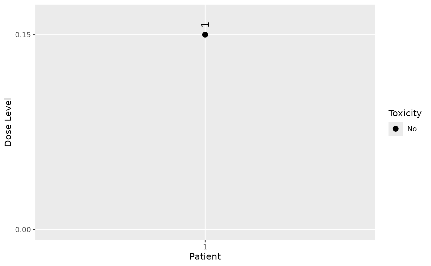
rm(list = c("x", "y", "ID", "cohort"))| ID | Cohort | Dose | DLT? |
|---|---|---|---|
| 1 | 1 | 0.15 | FALSE |
The dose grid is 0.15, 0.5, 1.5, 5, 15, 50, 150, 300, 600 and 900.
An overview of current DLT rate estimates
A quick summary and suggestion
First we update the model based on current accumulated data
res <- list()
with_progress({
    p <- progressor(length(scenario_list))
    for(s_idx in seq(length(scenario_list))){
        scenario_data <- scenario_list[[s_idx]]
        cur_res <- Test_Scenario(scenario_data,
                                 dose_grid = dose_grid,
                                 initial_model = initial_model,
                                 increment_rule = increment_rule,
                                 next_best_rule = next_best_rule,
                                 stop_rule = stop_rule,
                                 cohort_size_rule = cohort_size,
                                 mcmc_options = test_mcmc_options) %>%
            mutate(scenario = s_idx, .before = everything())
        res[[s_idx]] <- cur_res
        p(message = c("Scenario ", s_idx, " finished!"))
    }
})
table_c <- bind_rows(!!!res) %>%
    mutate(cohort_id = as.integer(cohort_id),
           treated = as.integer(treated),
           with_dlt = as.integer(with_dlt))
ft_res <- Flextable_TC(table_c, digits = 4, dose_unit = dose_unit)
ft_res
Scenario |
Cohort ID |
Dose (ug/kg) |
N |
Number of DLT |
Recommended Next Dose |
P(Target) |
P(Over) |
Median P(d) |
|---|---|---|---|---|---|---|---|---|
1 |
1 |
0.1500 |
1 |
0 |
0.5000 |
0.0525 |
0.0493 |
0.0077 |
We can give the current estimation of posterior distribution of DLT rate at the dose grid:
post_samples <- mcmc(data = current_data,
                     model = initial_model,
                     options = test_mcmc_options)
res <- sapply(
    dose_grid,
    Summary_crmPack_Samples,
    ref_dose = initial_model@ref_dose,
    samples = post_samples,
    prob_cut = prob_target_cut
)

post_res <- data.frame(dose = dose_grid, t(res))

ft_res <- Flextable_TB(
    post_res %>% select(-na_num),
    prob_target_cut,
    digits = 3,
    ewoc = ewoc_cut
)
ft_res
Dose |
Probability of DLT in |
Mean |
SD |
Quantiles |
||||
|---|---|---|---|---|---|---|---|---|
[0, 0.16) |
[0.16, 0.3) |
[0.3, 1] |
2.5% |
50% |
97.5% |
|||
0.150 |
0.920 |
0.043 |
0.037 |
0.044 |
0.102 |
0.000 |
0.005 |
0.359 |
0.500 |
0.898 |
0.052 |
0.049 |
0.054 |
0.115 |
0.000 |
0.008 |
0.417 |
1.500 |
0.870 |
0.066 |
0.064 |
0.067 |
0.129 |
0.000 |
0.012 |
0.487 |
5.000 |
0.828 |
0.084 |
0.088 |
0.087 |
0.148 |
0.000 |
0.021 |
0.560 |
15.000 |
0.775 |
0.102 |
0.123 |
0.112 |
0.171 |
0.000 |
0.035 |
0.644 |
50.000 |
0.687 |
0.134 |
0.179 |
0.153 |
0.200 |
0.000 |
0.063 |
0.739 |
150.000 |
0.579 |
0.151 |
0.270 |
0.213 |
0.235 |
0.002 |
0.115 |
0.830 |
300.000 |
0.484 |
0.162 |
0.354 |
0.270 |
0.262 |
0.004 |
0.172 |
0.888 |
600.000 |
0.391 |
0.161 |
0.448 |
0.341 |
0.296 |
0.006 |
0.246 |
0.953 |
900.000 |
0.351 |
0.153 |
0.496 |
0.381 |
0.313 |
0.008 |
0.295 |
0.977 |
*The doses in bold are not recommended as they do not meet EWOC criterion. | ||||||||
And a quick and rough visualization of DLT rate estimation
plot(post_samples, initial_model, current_data)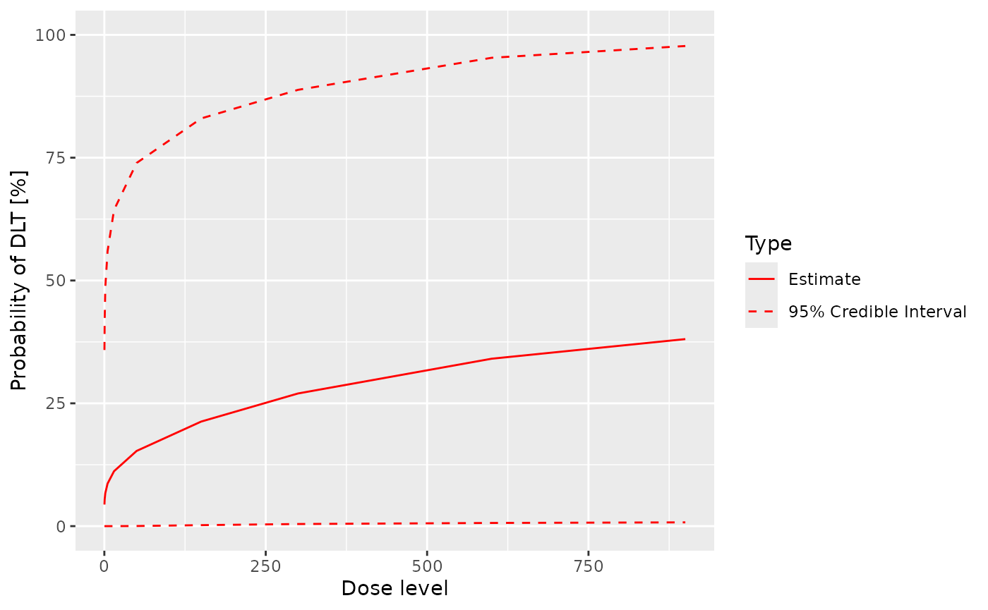
Summary code inspired by crmPack’s website
fullSamples <- getProbSamples(dose_grid, post_samples, initial_model)
fullSummary <- fullSamples %>%
  group_by(dose) %>%
  summarise(
    Mean = mean(prob),
    Median = median(prob),
    Q = list(quantile(prob, probs = c(0.05, 0.1, 0.25, 0.75, 0.9, 0.95), na.rm = TRUE))
  ) %>%
  unnest_wider(
    col = Q,
    names_repair = function(.x) {
      ifelse(
        str_detect(.x, "\\d+%"),
        sprintf("Q%02.0f", as.numeric(str_remove_all(.x, "%"))),
        .x
      )
    }
  )
#> Warning in sprintf("Q%02.0f", as.numeric(str_remove_all(.x, "%"))): NAs
#> introduced by coercion
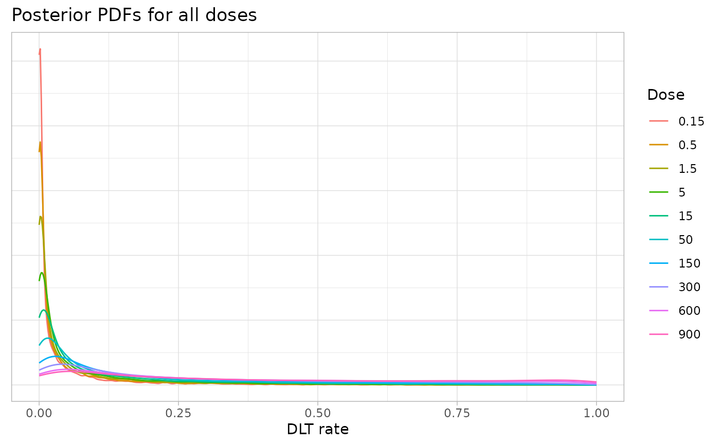
fullSamples %>%
  ggplot() +
  geom_line(aes(x = prob, color = as.factor(dose)),
            stat = "density") +
  theme_light() +
  theme(
    axis.text.y = element_blank(),
    axis.title.y = element_blank(),
    axis.ticks.y = element_blank()
  ) +
  labs(
    title = "Posterior PDFs for all doses",
    colour = "Dose",
    x = "DLT rate"
  )
# A simpler version of the visualization
# fullSummary %>%
# ggplot(aes(x = dose)) +
# geom_ribbon(aes(ymin = Q05, ymax = Q95), fill = "steelblue", alpha = 0.25) +
# geom_ribbon(aes(ymin = Q10, ymax = Q90), fill = "steelblue", alpha = 0.25) +
# geom_ribbon(aes(ymin = Q25, ymax = Q75), fill = "steelblue", alpha = 0.25) +
# geom_line(aes(y = Mean), colour = "black") +
# geom_line(aes(y = Median), colour = "blue") +
# theme_light() +
# labs(
# title = "Posterior Dose toxicity curve",
# colour = "Dose",
# y = "P(Toxicity)"
# )
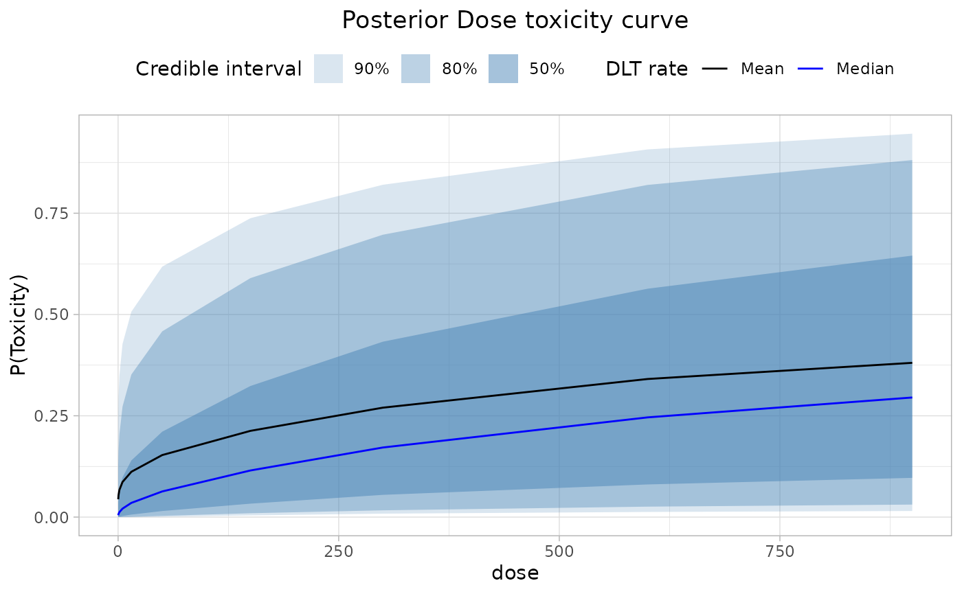
fullSummary %>%
rename(
ci90l = Q05,
ci90r = Q95,
ci80l = Q10,
ci80r = Q90,
ci50l = Q25,
ci50r = Q75
) %>%
pivot_longer(
cols = starts_with("ci"),
names_to = c("ci", ".value"),
names_pattern = "(ci[0-9]+)([l|r]+)",
) %>%
pivot_longer(
cols = c(Mean, Median),
names_to = "est_type",
values_to = "prob"
) %>%
ggplot(aes(x = dose)) +
geom_ribbon(
aes(ymin = l, ymax = r, alpha = ci),
fill = "steelblue"
) +
geom_line(aes(y = prob, color = est_type)) +
scale_color_manual(
values = c("black", "blue"),
breaks = c("Mean", "Median")
) +
scale_alpha_manual(
values = c(1 - 0.80 ^ 1,
1 - 0.80 ^ 2,
1 - 0.80 ^ 3),
breaks = c("ci90", "ci80", "ci50"),
labels = c("90%", "80%", "50%")
) +
theme_light() +
labs(
title = "Posterior Dose toxicity curve",
colour = "DLT rate",
y = "P(Toxicity)",
alpha = "Credible interval"
) +
theme(
legend.position = "top",
plot.title = element_text(hjust = 0.5)
)
Visualization code from my side
title_str <- paste0(
    "EWOC: post.pr. of excessive toxicity < ", formatC(ewoc_cut, digits = 2),
    "\n",
    "MTD: post.pr of target toxicity >= ", formatC(mtd_prob_target_thresh, digits = 2)
)
post_res %>%
    select(dose, under, target, over) %>%
    pivot_longer(cols = -dose,
                 names_to = "prob_type",
                 values_to = "prob") %>%
    mutate(dose_fct = factor(dose, levels = dose_grid)) %>%
    ggplot(aes(x = dose_fct, y = prob, color = prob_type, fill = prob_type)) +
    geom_col(position = "dodge") +
    geom_hline(
        yintercept = c(ewoc_cut, mtd_prob_target_thresh),
        linetype = "dashed"
    ) +
    scale_color_discrete(
        breaks = c("over", "target", "under"),
        labels = c("Excessive toxicity", "Target toxicity", "Under-dosing"),
        name = "Risk of DLT"
    ) +
    scale_fill_discrete(
        breaks = c("over", "target", "under"),
        labels = c("Excessive toxicity", "Target toxicity", "Under-dosing"),
        name = "Risk of DLT"
    ) +
    labs(
        x = "Dose",
        y = "Posterior probability",
        title = title_str) +
    theme_light()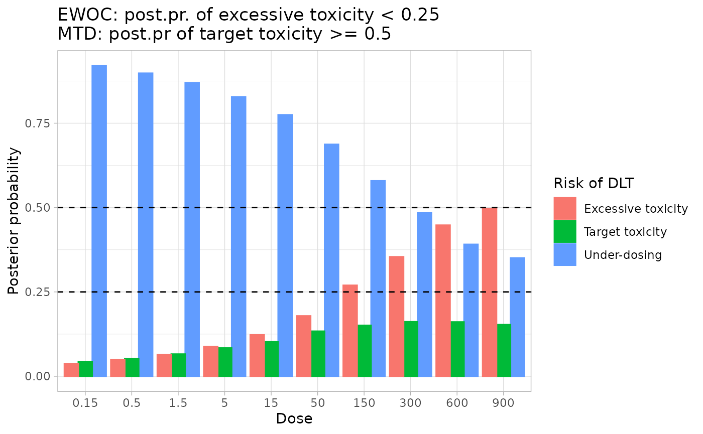
Visualization based on Haolin’s ref code
plot_list <- lapply(
    dose_grid,
    function(dose_pick, post_sample, post_res, prob_target_cut){
        fig <- Hist_And_Density(post_sample, dose_pick, post_res, prob_target_cut)
        return(fig)
        },
    post_sample = fullSamples,
    post_res = post_res,
    prob_target_cut = prob_target_cut)
cowplot::plot_grid(plotlist = plot_list, ncol = 2)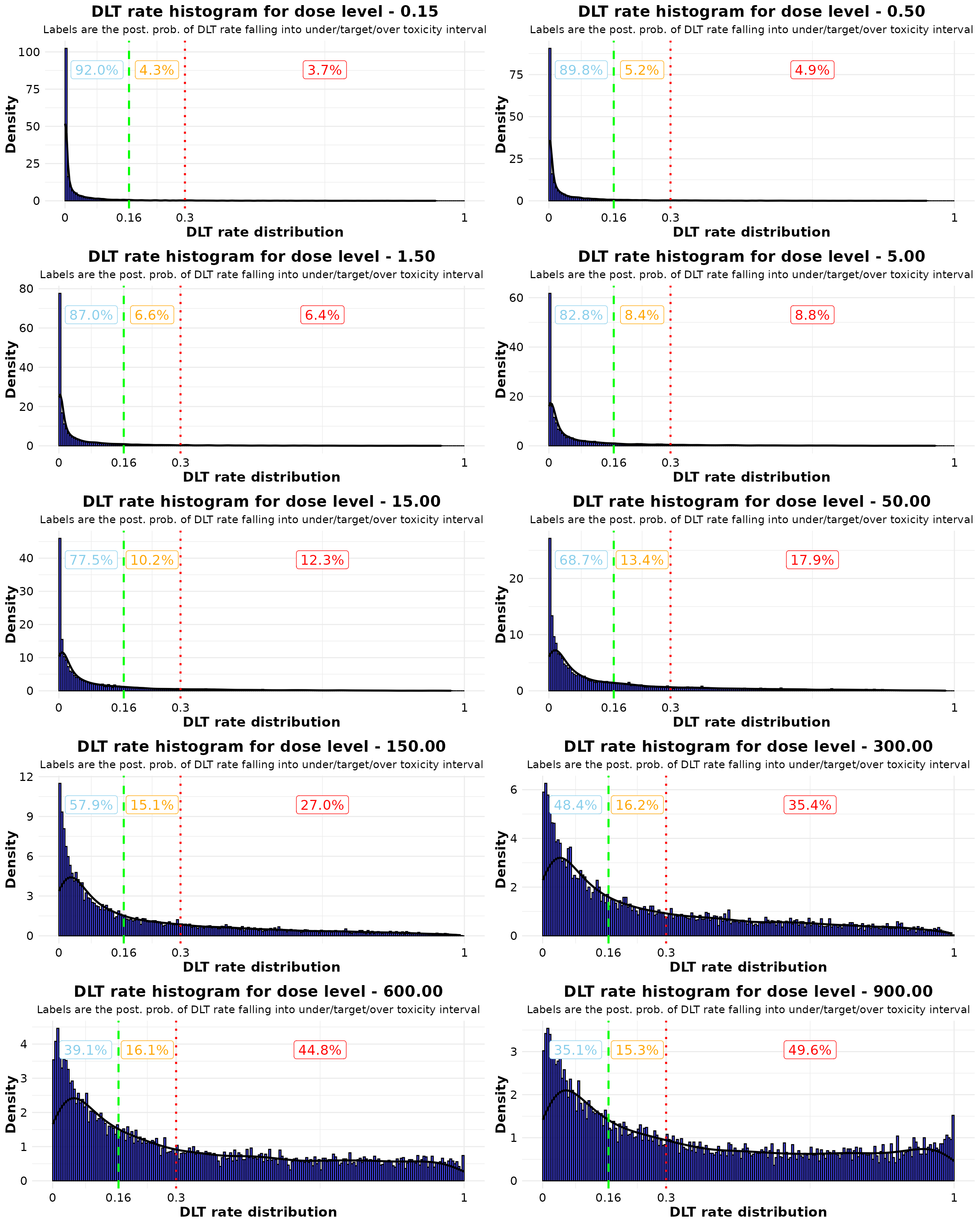
Make a recommendation
This section provides details about how we make the recommendation.
First compute the max does based on increment rule
# compute max feasible dose
next_max_dose <- maxDose(increment_rule, current_data)
Make dose/cohort size recommendation and check for trial status recommendation based on current data
# compute EWOC probabilities and determine feasible dose range using `nextBest()`
next_recommend <- nextBest(
        next_best_rule,
        doselimit = next_max_dose,
        samples = post_samples,
        model = initial_model,
        data = current_data
)

next_cohort_size <- size(cohort_size_rule,
                         dose = next_recommend$value,
                         data = current_data)

next_stop <- stopTrial(
    stopping = stop_rule,
    dose = next_recommend$value,
    samples = post_samples,
    model = initial_model,
    data = current_data
)
Here are some recommendation from the model:
-
The recommended next dose is 0.5 ug/kg with the following visualization:
plot(next_recommend$plot)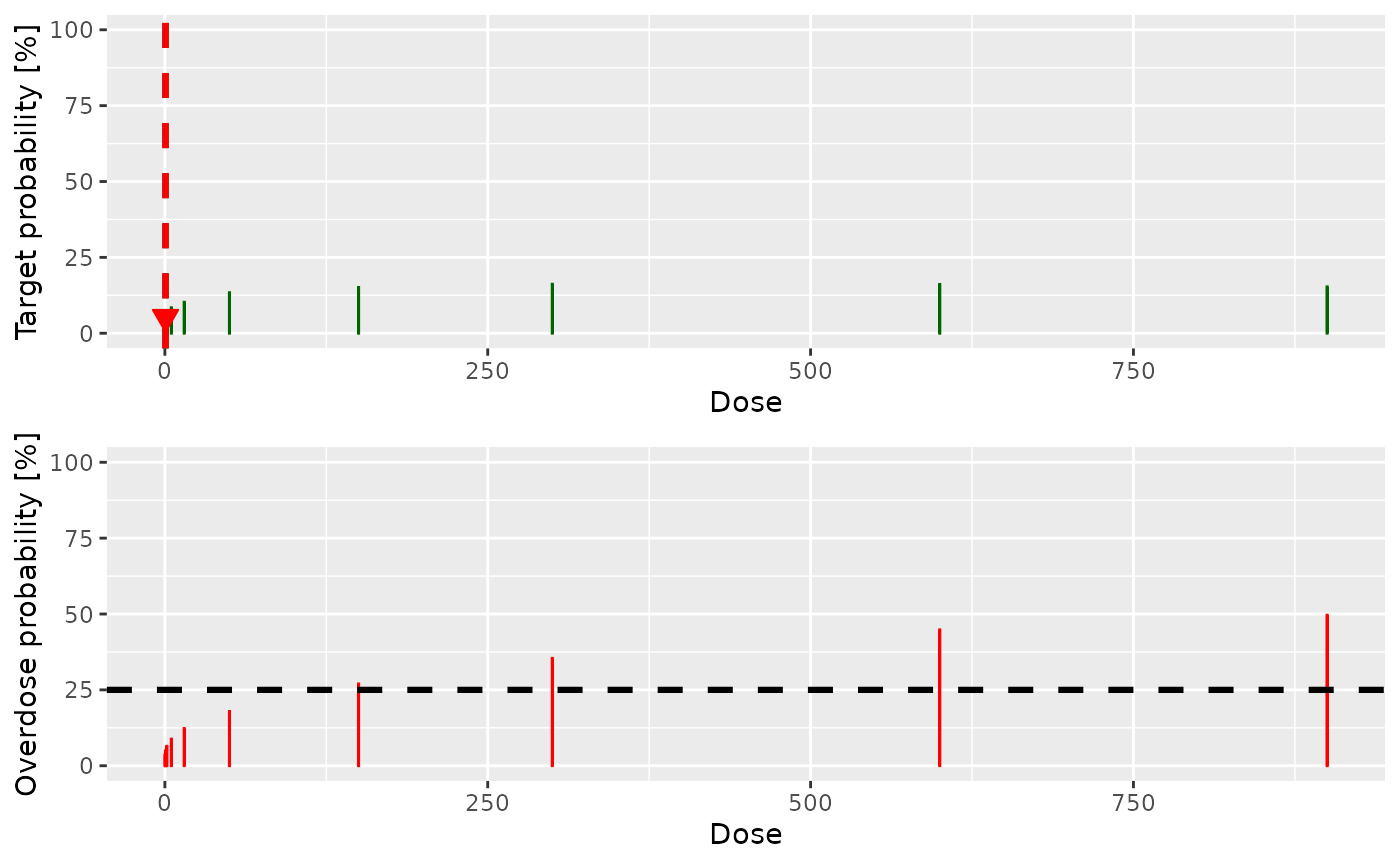
The recommended next cohort size is 1.
-
The trial is recommended to Continue with the detailed reason:
attr(next_stop, "message")
#> [[1]]
#> [1] "Number of patients is 1 and thus below the prespecified minimum number 90"
#>
#> [[2]]
#> [[2]][[1]]
#> [[2]][[1]][[1]]
#> [1] "0 patients lie within 0% of the next best dose 0.5. This is below the required 6 patients"
#>
#> [[2]][[1]][[2]]
#> [1] "Probability for target toxicity is 5 % for dose 0.5 and thus below the required 50 %"
#>
#>
#> [[2]][[2]]
#> [1] "0 patients lie within 0% of the next best dose 0.5. This is below the required 12 patients"
#>
#>
#> [[3]]
#> [1] "Next dose is available at the dose grid."
Also the full stopping rule is:
stop_any_full: If any of the following rules are
TRUE:max_subj_90: If 90 or more participants have been treated.
-
stop_any_mtd: If either of the following rules are
TRUE:-
stop_found_mtd: If both of the following rules are
TRUE:subj_at_mtd_6: If 6 or more participants have been treated at the next best dose.
dlt_prob_target_50%: If the probability of toxicity at the next best dose is in the range [0.16, 0.30] is at least 0.50.
subj_at_mtdmax_12: If 12 or more participants have been treated at the next best dose.
-
NA_recommend: If the dose returned by
nextBest()isNA, or if the trial includes a placebo dose, the placebo dose.
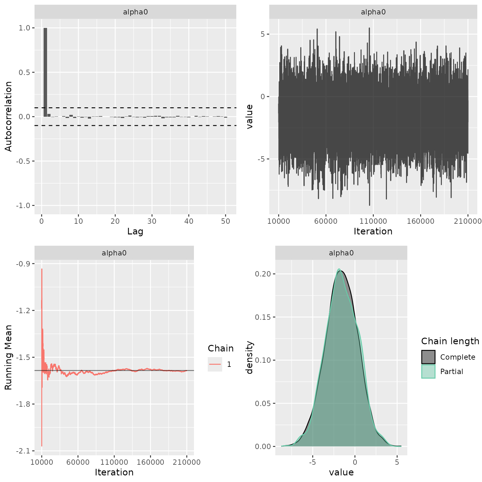
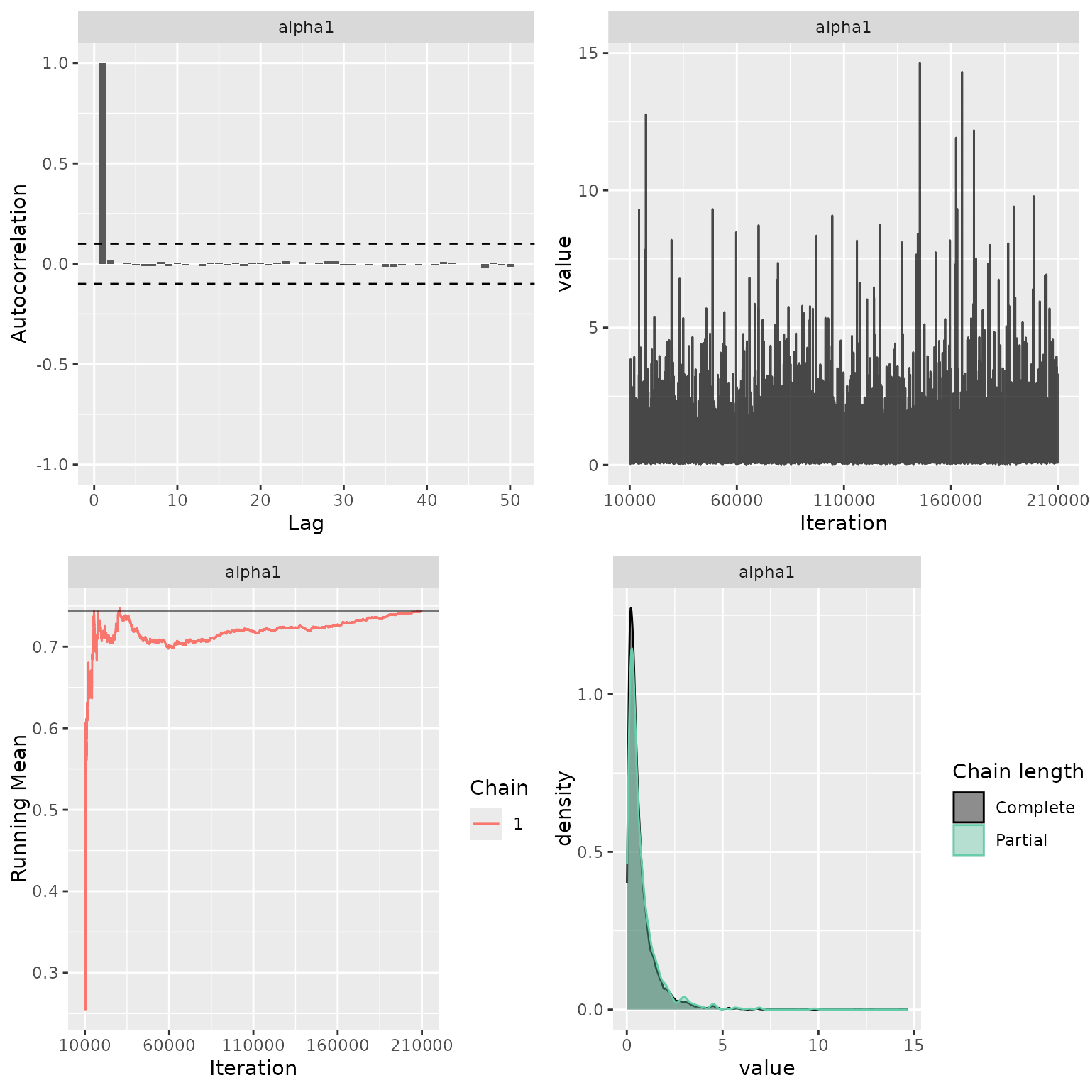
Sanity check of MCMC status
My_MCMC_Check <- function(indat){
    g1 <- ggs_autocorrelation(indat) +
        geom_hline(yintercept = c(-0.1, 0.1),
                   linetype = "dashed")

    g2 <- ggs_traceplot(indat)

    g3 <- ggs_running(indat)

    g4 <- ggs_compare_partial(indat)

    res <- cowplot::plot_grid(g1, g2, g3, g4, ncol = 2)

    return(res)
}
Appendix
Session info
#> ─ Session info ───────────────────────────────────────────────────────────────
#>  setting  value
#>  version  R version 4.4.1 (2024-06-14)
#>  os       Ubuntu 22.04.4 LTS
#>  system   x86_64, linux-gnu
#>  ui       X11
#>  language en
#>  collate  C.UTF-8
#>  ctype    C.UTF-8
#>  tz       UTC
#>  date     2024-08-06
#>  pandoc   3.1.11 @ /opt/hostedtoolcache/pandoc/3.1.11/x64/ (via rmarkdown)
#>
#> ─ Packages ───────────────────────────────────────────────────────────────────
#>  package           * version    date (UTC) lib source
#>  askpass             1.2.0      2023-09-03 [1] RSPM
#>  backports           1.5.0      2024-05-23 [1] RSPM
#>  BLRMeval          * 0.0.0.9005 2024-08-06 [1] local
#>  bslib               0.8.0      2024-07-29 [1] RSPM
#>  cachem              1.1.0      2024-05-16 [1] RSPM
#>  checkmate           2.3.2      2024-07-29 [1] RSPM
#>  cli                 3.6.3      2024-06-21 [1] RSPM
#>  coda                0.19-4.1   2024-01-31 [1] RSPM
#>  colorspace          2.1-1      2024-07-26 [1] RSPM
#>  cowplot             1.1.3      2024-01-22 [1] RSPM
#>  crayon              1.5.3      2024-06-20 [1] RSPM
#>  crmPack           * 2.0.0.9158 2024-08-05 [1] Github (openpharma/crmPack@75659a9)
#>  crul                1.5.0      2024-07-19 [1] RSPM
#>  curl                5.2.1      2024-03-01 [1] RSPM
#>  data.table          1.15.4     2024-03-30 [1] RSPM
#>  desc                1.4.3      2023-12-10 [1] RSPM
#>  digest              0.6.36     2024-06-23 [1] RSPM
#>  dplyr             * 1.1.4      2023-11-17 [1] RSPM
#>  evaluate            0.24.0     2024-06-10 [1] RSPM
#>  fansi               1.0.6      2023-12-08 [1] RSPM
#>  farver              2.1.2      2024-05-13 [1] RSPM
#>  fastmap             1.2.0      2024-05-15 [1] RSPM
#>  flextable         * 0.9.6      2024-05-05 [1] RSPM
#>  fontBitstreamVera   0.1.1      2017-02-01 [1] RSPM
#>  fontLiberation      0.1.0      2016-10-15 [1] RSPM
#>  fontquiver          0.2.1      2017-02-01 [1] RSPM
#>  forcats           * 1.0.0      2023-01-29 [1] RSPM
#>  formatR             1.14       2023-01-17 [1] RSPM
#>  fs                  1.6.4      2024-04-25 [1] RSPM
#>  futile.logger       1.4.3      2016-07-10 [1] RSPM
#>  futile.options      1.0.1      2018-04-20 [1] RSPM
#>  gdtools             0.3.7      2024-03-05 [1] RSPM
#>  generics            0.1.3      2022-07-05 [1] RSPM
#>  GenSA               1.1.14     2024-01-22 [1] RSPM
#>  gfonts              0.2.0      2023-01-08 [1] RSPM
#>  GGally              2.2.1      2024-02-14 [1] RSPM
#>  ggmcmc            * 1.5.1.1    2021-02-10 [1] RSPM
#>  ggplot2           * 3.5.1      2024-04-23 [1] RSPM
#>  ggstats             0.6.0      2024-04-05 [1] RSPM
#>  glue                1.7.0      2024-01-09 [1] RSPM
#>  gridExtra           2.3        2017-09-09 [1] RSPM
#>  gtable              0.3.5      2024-04-22 [1] RSPM
#>  highr               0.11       2024-05-26 [1] RSPM
#>  hms                 1.1.3      2023-03-21 [1] RSPM
#>  htmltools           0.5.8.1    2024-04-04 [1] RSPM
#>  htmlwidgets         1.6.4      2023-12-06 [1] RSPM
#>  httpcode            0.3.0      2020-04-10 [1] RSPM
#>  httpuv              1.6.15     2024-03-26 [1] RSPM
#>  jquerylib           0.1.4      2021-04-26 [1] RSPM
#>  jsonlite            1.8.8      2023-12-04 [1] RSPM
#>  kableExtra          1.4.0      2024-01-24 [1] RSPM
#>  knitr               1.48       2024-07-07 [1] RSPM
#>  labeling            0.4.3      2023-08-29 [1] RSPM
#>  lambda.r            1.2.4      2019-09-18 [1] RSPM
#>  later               1.3.2      2023-12-06 [1] RSPM
#>  lattice             0.22-6     2024-03-20 [3] CRAN (R 4.4.1)
#>  lifecycle           1.0.4      2023-11-07 [1] RSPM
#>  lubridate         * 1.9.3      2023-09-27 [1] RSPM
#>  magrittr            2.0.3      2022-03-30 [1] RSPM
#>  mime                0.12       2021-09-28 [1] RSPM
#>  munsell             0.5.1      2024-04-01 [1] RSPM
#>  mvtnorm             1.2-5      2024-05-21 [1] RSPM
#>  officer             0.6.6      2024-05-05 [1] RSPM
#>  openssl             2.2.0      2024-05-16 [1] RSPM
#>  parallelly          1.38.0     2024-07-27 [1] RSPM
#>  pillar              1.9.0      2023-03-22 [1] RSPM
#>  pkgconfig           2.0.3      2019-09-22 [1] RSPM
#>  pkgdown             2.1.0      2024-07-06 [1] any (@2.1.0)
#>  plyr                1.8.9      2023-10-02 [1] RSPM
#>  progressr         * 0.14.0     2023-08-10 [1] RSPM
#>  promises            1.3.0      2024-04-05 [1] RSPM
#>  purrr             * 1.0.2      2023-08-10 [1] RSPM
#>  R6                  2.5.1      2021-08-19 [1] RSPM
#>  ragg                1.3.2      2024-05-15 [1] RSPM
#>  RColorBrewer        1.1-3      2022-04-03 [1] RSPM
#>  Rcpp                1.0.13     2024-07-17 [1] RSPM
#>  readr             * 2.1.5      2024-01-10 [1] RSPM
#>  rjags               4-15       2023-11-30 [1] RSPM
#>  rlang               1.1.4      2024-06-04 [1] RSPM
#>  rmarkdown           2.27       2024-05-17 [1] RSPM
#>  rstudioapi          0.16.0     2024-03-24 [1] RSPM
#>  sass                0.4.9      2024-03-15 [1] RSPM
#>  scales              1.3.0      2023-11-28 [1] RSPM
#>  sessioninfo         1.2.2      2021-12-06 [1] RSPM
#>  shiny               1.9.1      2024-08-01 [1] RSPM
#>  stringi             1.8.4      2024-05-06 [1] RSPM
#>  stringr           * 1.5.1      2023-11-14 [1] RSPM
#>  svglite             2.1.3      2023-12-08 [1] RSPM
#>  systemfonts         1.1.0      2024-05-15 [1] RSPM
#>  textshaping         0.4.0      2024-05-24 [1] RSPM
#>  tibble            * 3.2.1      2023-03-20 [1] RSPM
#>  tidyr             * 1.3.1      2024-01-24 [1] RSPM
#>  tidyselect          1.2.1      2024-03-11 [1] RSPM
#>  tidyverse         * 2.0.0      2023-02-22 [1] any (@2.0.0)
#>  timechange          0.3.0      2024-01-18 [1] RSPM
#>  tzdb                0.4.0      2023-05-12 [1] RSPM
#>  utf8                1.2.4      2023-10-22 [1] RSPM
#>  uuid                1.2-1      2024-07-29 [1] RSPM
#>  vctrs               0.6.5      2023-12-01 [1] RSPM
#>  viridisLite         0.4.2      2023-05-02 [1] RSPM
#>  withr               3.0.1      2024-07-31 [1] RSPM
#>  xfun                0.46       2024-07-18 [1] RSPM
#>  xml2                1.3.6      2023-12-04 [1] RSPM
#>  xtable              1.8-4      2019-04-21 [1] RSPM
#>  yaml                2.3.10     2024-07-26 [1] RSPM
#>  zip                 2.3.1      2024-01-27 [1] RSPM
#>
#>  [1] /home/runner/work/_temp/Library
#>  [2] /opt/R/4.4.1/lib/R/site-library
#>  [3] /opt/R/4.4.1/lib/R/library
#>
#> ──────────────────────────────────────────────────────────────────────────────